Die Nutanix Bibel

Copyright (c) 2016: Die Nutanix Bibel und nutanix-bibel.com, 2016. Unauthorized use and/or duplication of this material without express and written permission from this blog’s author and/or owner is strictly prohibited. Excerpts and links may be used, provided that full and clear credit is given to Steven Poitras and nutanix-bibel.com with appropriate and specific direction to the original content.
Haben Sie Feedback für uns? Haben Sie einen Schreibfehler gefunden? Schicken Sie Ihr Feedback an: admin at nutanix-bibel punkt com
Übersetzungen stehen zur Verfügung:


Eine PDF Version steht zur Verfügung (Hinweis: nicht alle Aktualisierungen der Seite sind in der PDF Version enthalten):

Einführung

Dheeraj Pandey, CEO, Nutanix
Ich freue mich eine Einleitung für dieses Buch schreiben zu dürfen, dass inzwischen bei fast allen bekannt geworden ist als "Die Nutanix Bibel". Als erstes möchte ich den Titel des Buches ansprechen, welches manche Personen vielleicht in betracht ihrer eigenen Religion als ein wenig respektlos betrachten würden. Es gibt eine Erklärung in das Wörterbuch von Merriam Webster für die Bedeutung des Wortes "Bibel", die sich nicht wortwörtlich auf die Heilige Schrift bezieht: "eine Schrift, die vor allem in sachen Autorität, oder durch Ihre breite Leserschaft, als führend betrachtet werden kann". ----- Und genau so sollte man seine Wurzeln interpretieren. Es fing an, von einem der bescheidensten und zugleich kenntnisreichen Mitarbeiter von Nutanix, Steven Poitras, unserem ersten Solution Architect, geschrieben zu werden, der weiterhin maßgeblich zu diesem Thema ist, ohne seine "frühe Angestellter" -Untermodalität auszuführen. Wissen zu ihm war nicht Macht - die Tat des Teilens dieses Wissens ist, was ihn in diesem Unternehmen herausragend macht. Steve verkörpert Kultur in diesem Unternehmen - indem er jedem anderen mit seiner Autorität zu diesem Thema hilft, indem er ihnen hilft, ihre Aufgaben in Power Shell oder Python zu automatisieren, indem sie aufwendige Referenzarchitekturen aufbaut, die sowohl inhaltlich als auch formal ausgewogen sind Ein Echtzeit-Kumpel für alle, die Hilfe auf Yammer oder Twitter, indem sie transparent mit Ingenieuren auf die Notwendigkeit, Selbstreflexion und Selbst-Verbesserung, und durch ehrgeizige.
When he came forward to write a blog, his big dream was to lead with transparency, and to build advocates in the field who would be empowered to make design trade-offs based on this transparency. It is rare for companies to open up on design and architecture as much as Steve has with his blog. Most open source companies -- who at the surface might seem transparent because their code is open source -- never talk in-depth about design, and "how it works" under the hood. When our competitors know about our product or design weaknesses, it makes us stronger -- because there is very little to hide, and everything to gain when something gets critiqued under a crosshair. A public admonition of a feature trade-off or a design decision drives the entire company on Yammer in quick time, and before long, we've a conclusion on whether it is a genuine weakness or a true strength that someone is fear-mongering on. Nutanix Bible, in essence, protects us from drinking our own kool aid. That is the power of an honest discourse with our customers and partners.
This ever-improving artifact, beyond being authoritative, is also enjoying wide readership across the world. Architects, managers, and CIOs alike, have stopped me in conference hallways to talk about how refreshingly lucid the writing style is, with some painfully detailed illustrations, visio diagrams, and pictorials. Steve has taken time to tell the web-scale story, without taking shortcuts. Democratizing our distributed architecture was not going to be easy in a world where most IT practitioners have been buried in dealing with the "urgent". The Bible bridges the gap between IT and DevOps, because it attempts to explain computer science and software engineering trade-offs in very simple terms. We hope that in the coming 3-5 years, IT will speak a language that helps them get closer to the DevOps' web-scale jargon.
With this first edition, we are converting Steve's blog into a book. The day we stop adding to this book is the beginning of the end of this company. I expect each and everyone of you to keep reminding us of what brought us this far: truth, the whole truth, and nothing but the truth, will set you free (from complacency and hubris).
Keep us honest.
--Dheeraj Pandey, CEO, Nutanix

Stuart Miniman, Principal Research Contributor, Wikibon
Users today are constantly barraged by new technologies. There is no limit of new opportunities for IT to change to a "new and better way", but the adoption of new technology and more importantly, the change of operations and processes is difficult. Even the huge growth of open source technologies has been hampered by lack of adequate documentation. Wikibon was founded on the principal that the community can help with this problem and in that spirit, Die Nutanix Bibel, which started as a blog post by Steve Poitras, has become a valuable reference point for IT practitioners that want to learn about hypercovergence and web-scale principles or to dig deep into Nutanix and hypervisor architectures. The concepts that Steve has written about are advanced software engineering problems that some of the smartest engineers in the industry have designed a solution for. The book explains these technologies in a way that is understandable to IT generalists without compromising the technical veracity.
The concepts of distributed systems and software-led infrastructure are critical for IT practitioners to understand. I encourage both Nutanix customers and everyone who wants to understand these trends to read the book. The technologies discussed here power some of the largest datacenters in the world.
--Stuart Miniman, Principal Research Contributor, Wikibon
Introduction
Steven Poitras, Principal Solutions Architect, Nutanix
Welcome to Die Nutanix Bibel! I work with the Nutanix platform on a daily basis – trying to find issues, push its limits as well as administer it for my production benchmarking lab. This item is being produced to serve as a living document outlining tips and tricks used every day by myself and a variety of engineers here at Nutanix.
NOTE: What you see here is an under the covers look at how things work. With that said, all topics discussed are abstracted by Nutanix and knowledge isn't required to successfully operate a Nutanix environment!
Enjoy!
--Steven Poitras, Principal Solutions Architect, Nutanix
Part I. A Brief Lesson in History
A brief look at the history of infrastructure and what has led us to where we are today.
The Evolution of the Datacenter
The datacenter has evolved significantly over the last several decades. The following sections will examine each era in detail.
The Era of the Mainframe
The mainframe ruled for many years and laid the core foundation of where we are today. It allowed companies to leverage the following key characteristics:
- Natively converged CPU, main memory, and storage
- Engineered internal redundancy
But the mainframe also introduced the following issues:
- The high costs of procuring infrastructure
- Inherent complexity
- A lack of flexibility and highly siloed environments
The Move to Stand-Alone Servers
With mainframes, it was very difficult for organizations within a business to leverage these capabilities which partly led to the entrance of pizza boxes or stand-alone servers. Key characteristics of stand-alone servers included:
- CPU, main memory, and DAS storage
- Higher flexibility than the mainframe
- Accessed over the network
These stand-alone servers introduced more issues:
- Increased number of silos
- Low or unequal resource utilization
- The server became a single point of failure (SPOF) for both compute AND storage
Centralized Storage
Businesses always need to make money and data is a key piece of that puzzle. With direct-attached storage (DAS), organizations either needed more space than was locally available, or data high availability (HA) where a server failure wouldn’t cause data unavailability.
Centralized storage replaced both the mainframe and the stand-alone server with sharable, larger pools of storage that also provided data protection. Key characteristics of centralized storage included:
- Pooled storage resources led to better storage utilization
- Centralized data protection via RAID eliminated the chance that server loss caused data loss
- Storage were performed over the network
Issues with centralized storage included:
- They were potentially more expensive, however data is more valuable than the hardware
- Increased complexity (SAN Fabric, WWPNs, RAID groups, volumes, spindle counts, etc.)
- They required another management tool / team
The Introduction of Virtualization
At this point in time, compute utilization was low and resource efficiency was impacting the bottom line. Virtualization was then introduced and enabled multiple workloads and operating systems (OSs) to run as virtual machines (VMs) on a single piece of hardware. Virtualization enabled businesses to increase utilization of their pizza boxes, but also increased the number of silos and the impacts of an outage. Key characteristics of virtualization included:
- Abstracting the OS from hardware (VM)
- Very efficient compute utilization led to workload consolidation
Issues with virtualization included:
- An increase in the number of silos and management complexity
- A lack of VM high-availability, so if a compute node failed the impact was much larger
- A lack of pooled resources
- The need for another management tool / team
Virtualization Matures
The hypervisor became a very efficient and feature-filled solution. With the advent of tools, including VMware vMotion, HA, and DRS, users obtained the ability to provide VM high availability and migrate compute workloads dynamically. The only caveat was the reliance on centralized storage, causing the two paths to merge. The only down turn was the increased load on the storage array before and VM sprawl led to contention for storage I/O. Key characteristics included:
- Clustering led to pooled compute resources
- The ability to dynamically migrate workloads between compute nodes (DRS / vMotion)
- The introduction of VM high availability (HA) in the case of a compute node failure
- A requirement for centralized storage
Issues included:
- Higher demand on storage due to VM sprawl
- Requirements to scale out more arrays creating more silos and more complexity
- Higher $ / GB due to requirement of an array
- The possibility of resource contention on array
- It made storage configuration much more complex due to the necessity to ensure:
- VM to datastore / LUN ratios
- Spindle count to facilitate I/O requirements
Solid State Disks (SSDs)
SSDs helped alleviate this I/O bottleneck by providing much higher I/O performance without the need for tons of disk enclosures. However, given the extreme advances in performance, the controllers and network had not yet evolved to handle the vast I/O available. Key characteristics of SSDs included:
- Much higher I/O characteristics than traditional HDD
- Essentially eliminated seek times
SSD issues included:
- The bottleneck shifted from storage I/O on disk to the controller / network
- Silos still remained
- Array configuration complexity still remained
In Comes Cloud
The term cloud can be very ambiguous by definition. Simply put it's the ability to consume and leverage a service hosted somewhere provided by someone else.
With the introduction of cloud, the perspectives IT, the business and end-users have shifted.
Business groups and IT consumers require IT provide the same capabilities of cloud, its agility and time to value. If not, they will go directly to cloud which causes another issue for IT: data security.
Core pillars of any cloud service:
-
Self-service / On-demand
- Rapid time to value (TTV) / little barrier to entry
-
Service and SLA focus
- Contractual guarantees around uptime / availability / performance
-
Fractional consumption model
- Pay for what you use (some services are free)
Cloud Classifications
Most general classifications of cloud fall into three main buckets (starting at the highest level and moving downward):
-
Software as a Service (SaaS)
- Any software / service consumed via a simple url
- Examples: Workday, Salesforce.com, Google search, etc.
-
Platform as a Service (PaaS)
- Development and deployment platform
- Examples: Amazon Elastic Beanstalk / Relational Database Services (RDS), Google App Engine, etc.
-
Infrastructure as a Service (IaaS)
- VMs/Containers/NFV as a service
- Examples: Amazon EC2/ECS, Microsoft Azure, Google Compute Engine (GCE), etc.
Shift in IT focus
Cloud poses an interesting dilemma for IT. They can embrace it, or they can try to provide an alternative. They want to keep the data internal, but need to allow for the self-service, rapid nature of cloud.
This shift forces IT to act more as a legitimate service provider to their end-users (company employees).
The Importance of Latency
The figure below characterizes the various latencies for specific types of I/O:
| Item | Latency | Comments |
|---|---|---|
| L1 cache reference | 0.5 ns | |
| L2 cache reference | 7 ns | 14x L1 cache |
| DRAM access | 100 ns | 20x L2 cache, 200x L1 cache |
| 3D XPoint based NVMe SSD read | 00's of ns (expected) | .1 us or 0.01 ms (expected) |
| NAND NVMe SSD R/W | 20,000 ns | 20 us or 0.02 ms |
| NAND SATA SSD R/W | 50,000-60,000 ns | 50-60 us or 0.05-0.06 ms |
| Read 4K randomly from SSD | 150,000 ns | 150 us or 0.15 ms |
| Read 1MB sequentially from memory | 250,000 ns | 250 us or 0.25 ms |
| Round trip within datacenter | 500,000 ns | 500 us or 0.5 ms |
| Read 1MB sequentially from SSD | 1,000,000 ns | 1 ms, 4x memory |
| Disk seek | 10,000,000 ns or 10,000 us | 10 ms, 20x datacenter round trip |
| Read 1MB sequentially from disk | 20,000,000 ns or 20,000 us | 20 ms, 80x memory, 20x SSD |
| Send packet CA -> Netherlands -> CA | 150,000,000 ns | 150 ms |
(credit: Jeff Dean, https://gist.github.com/jboner/2841832)
The table above shows that the CPU can access its caches at anywhere from ~0.5-7ns (L1 vs. L2). For main memory, these accesses occur at ~100ns, whereas a local 4K SSD read is ~150,000ns or 0.15ms.
If we take a typical enterprise-class SSD (in this case the Intel S3700 - SPEC), this device is capable of the following:
- Random I/O performance:
- Random 4K Reads: Up to 75,000 IOPS
- Random 4K Writes: Up to 36,000 IOPS
- Sequential bandwidth:
- Sustained Sequential Read: Up to 500MB/s
- Sustained Sequential Write: Up to 460MB/s
- Latency:
- Read: 50us
- Write: 65us
Looking at the Bandwidth
For traditional storage, there are a few main types of media for I/O:
- Fiber Channel (FC)
- 4-, 8-, and 16-Gb
- Ethernet (including FCoE)
- 1-, 10-Gb, (40-Gb IB), etc.
For the calculation below, we are using the 500MB/s Read and 460MB/s Write BW available from the Intel S3700.
The calculation is done as follows:
numSSD = ROUNDUP((numConnections * connBW (in GB/s))/ ssdBW (R or W))
NOTE: Numbers were rounded up as a partial SSD isn’t possible. This also does not account for the necessary CPU required to handle all of the I/O and assumes unlimited controller CPU power.
| Network BW | SSDs required to saturate network BW | ||
|---|---|---|---|
| Controller Connectivity | Available Network BW | Read I/O | Write I/O |
| Dual 4Gb FC | 8Gb == 1GB | 2 | 3 |
| Dual 8Gb FC | 16Gb == 2GB | 4 | 5 |
| Dual 16Gb FC | 32Gb == 4GB | 8 | 9 |
| Dual 1Gb ETH | 2Gb == 0.25GB | 1 | 1 |
| Dual 10Gb ETH | 20Gb == 2.5GB | 5 | 6 |
As the table shows, if you wanted to leverage the theoretical maximum performance an SSD could offer, the network can become a bottleneck with anywhere from 1 to 9 SSDs depending on the type of networking leveraged
The Impact to Memory Latency
Typical main memory latency is ~100ns (will vary), we can perform the following calculations:
- Local memory read latency = 100ns + [OS / hypervisor overhead]
- Network memory read latency = 100ns + NW RTT latency + [2 x OS / hypervisor overhead]
If we assume a typical network RTT is ~0.5ms (will vary by switch vendor) which is ~500,000ns that would come down to:
- Network memory read latency = 100ns + 500,000ns + [2 x OS / hypervisor overhead]
If we theoretically assume a very fast network with a 10,000ns RTT:
- Network memory read latency = 100ns + 10,000ns + [2 x OS / hypervisor overhead]
What that means is even with a theoretically fast network, there is a 10,000% overhead when compared to a non-network memory access. With a slow network this can be upwards of a 500,000% latency overhead.
In order to alleviate this overhead, server side caching technologies are introduced.
Book of Web-Scale
web·scale - /web ' skãl/ - noun - computing architecture
a new architectural approach to infrastructure and computing.
This section will present some of the core concepts behind “Web-scale” infrastructure and why we leverage them. Before I get started, I just wanted to clearly state the Web-scale doesn’t mean you need to be “web-scale” (e.g. Google, Facebook, or Microsoft). These constructs are applicable and beneficial at any scale (3-nodes or thousands of nodes).
Historical challenges included:
- Complexity, complexity, complexity
- Desire for incremental based growth
- The need to be agile
There are a few key constructs used when talking about “Web-scale” infrastructure:
- Hyper-convergence
- Software defined intelligence
- Distributed autonomous systems
- Incremental and linear scale out
Other related items:
- API-based automation and rich analytics
- Self-healing
The following sections will provide a technical perspective on what they actually mean.
Hyper-Convergence
There are differing opinions on what hyper-convergence actually is. It also varies based on the scope of components (e.g. virtualization, networking, etc.). However, the core concept comes down to the following: natively combining two or more components into a single unit. ‘Natively’ is the key word here. In order to be the most effective, the components must be natively integrated and not just bundled together. In the case of Nutanix, we natively converge compute + storage to form a single node used in our appliance. For others, this might be converging storage with the network, etc. What it really means:
- Natively integrating two or more components into a single unit which can be easily scaled
Benefits include:
- Single unit to scale
- Localized I/O
- Eliminates traditional compute / storage silos by converging them
Software-Defined Intelligence
Software-defined intelligence is taking the core logic from normally proprietary or specialized hardware (e.g. ASIC / FPGA) and doing it in software on commodity hardware. For Nutanix, we take the traditional storage logic (e.g. RAID, deduplication, compression, etc.) and put that into software that runs in each of the Nutanix Controller VMs (CVM) on standard x86 hardware. What it really means:
- Pulling key logic from hardware and doing it in software on commodity hardware
Benefits include:
- Rapid release cycles
- Elimination of proprietary hardware reliance
- Utilization of commodity hardware for better economics
Distributed Autonomous Systems
Distributed autonomous systems involve moving away from the traditional concept of having a single unit responsible for doing something and distributing that role among all nodes within the cluster. You can think of this as creating a purely distributed system. Traditionally, vendors have assumed that hardware will be reliable, which, in most cases can be true. However, core to distributed systems is the idea that hardware will eventually fail and handling that fault in an elegant and non-disruptive way is key.
These distributed systems are designed to accommodate and remediate failure, to form something that is self-healing and autonomous. In the event of a component failure, the system will transparently handle and remediate the failure, continuing to operate as expected. Alerting will make the user aware, but rather than being a critical time-sensitive item, any remediation (e.g. replace a failed node) can be done on the admin’s schedule. Another way to put it is fail in-place (rebuild without replace) For items where a “master” is needed an election process is utilized, in the event this master fails a new master is elected. To distribute the processing of tasks MapReduce concepts are leveraged. What it really means:
- Distributing roles and responsibilities to all nodes within the system
- Utilizing concepts like MapReduce to perform distributed processing of tasks
- Using an election process in the case where a “master” is needed
Benefits include:
- Eliminates any single points of failure (SPOF)
- Distributes workload to eliminate any bottlenecks
Incremental and linear scale out
Incremental and linear scale out relates to the ability to start with a certain set of resources and as needed scale them out while linearly increasing the performance of the system. All of the constructs mentioned above are critical enablers in making this a reality. For example, traditionally you’d have 3-layers of components for running virtual workloads: servers, storage, and network – all of which are scaled independently. As an example, when you scale out the number of servers you’re not scaling out your storage performance. With a hyper-converged platform like Nutanix, when you scale out with new node(s) you’re scaling out:
- The number of hypervisor / compute nodes
- The number of storage controllers
- The compute and storage performance / capacity
- The number of nodes participating in cluster wide operations
What it really means:
- The ability to incrementally scale storage / compute with linear increases to performance / ability
Benefits include:
- The ability to start small and scale
- Uniform and consistent performance at any scale
Making Sense of It All
In summary:
- Inefficient compute utilization led to the move to virtualization
- Features including vMotion, HA, and DRS led to the requirement of centralized storage
- VM sprawl led to the increase load and contention on storage
- SSDs came in to alleviate the issues but changed the bottleneck to the network / controllers
- Cache / memory accesses over the network face large overheads, minimizing their benefits
- Array configuration complexity still remains the same
- Server side caches were introduced to alleviate the load on the array / impact of the network, however introduces another component to the solution
- Locality helps alleviate the bottlenecks / overheads traditionally faced when going over the network
- Shifts the focus from infrastructure to ease of management and simplifying the stack
- The birth of the Web-Scale world!
Part II. Book of Prism
prism - /'prizɘm/ - noun - control plane
one-click management and interface for datacenter operations.
Design Methodology and Iterations
Building a beautiful, empathetic and intuitive product are core to the Nutanix platform and something we take very seriously. This section will cover our design methodology and how we iterate on them. More coming here soon!
In the meantime feel free to check out this great post on our design methodology and iterations by our Product Design Lead, Jeremy Sallee (who also designed this) - http://salleedesign.com/stuff/sdwip/blog/nutanix-case-study/
You can download the Nutanix Visio stencils here: http://www.visiocafe.com/nutanix.htm
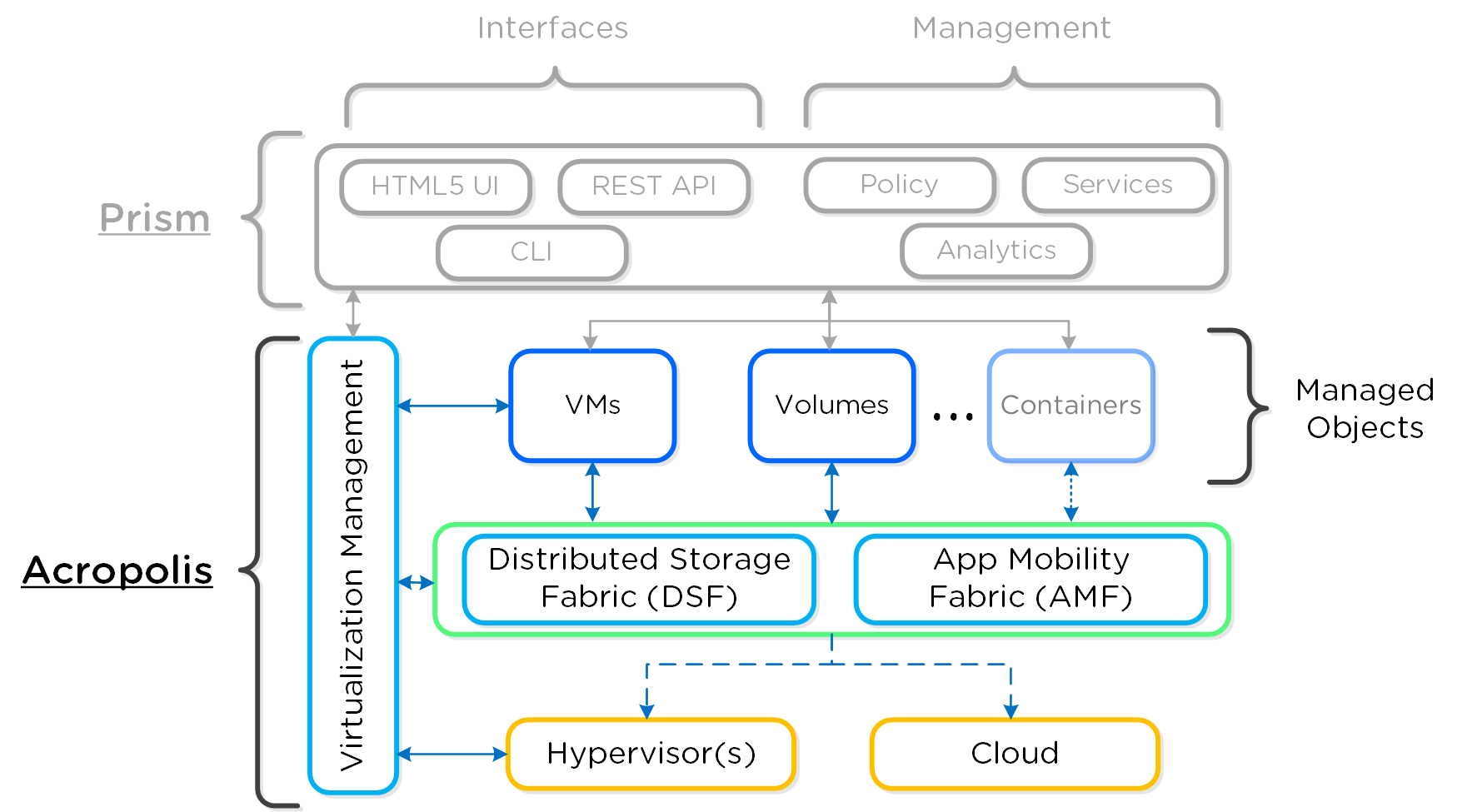
Architecture
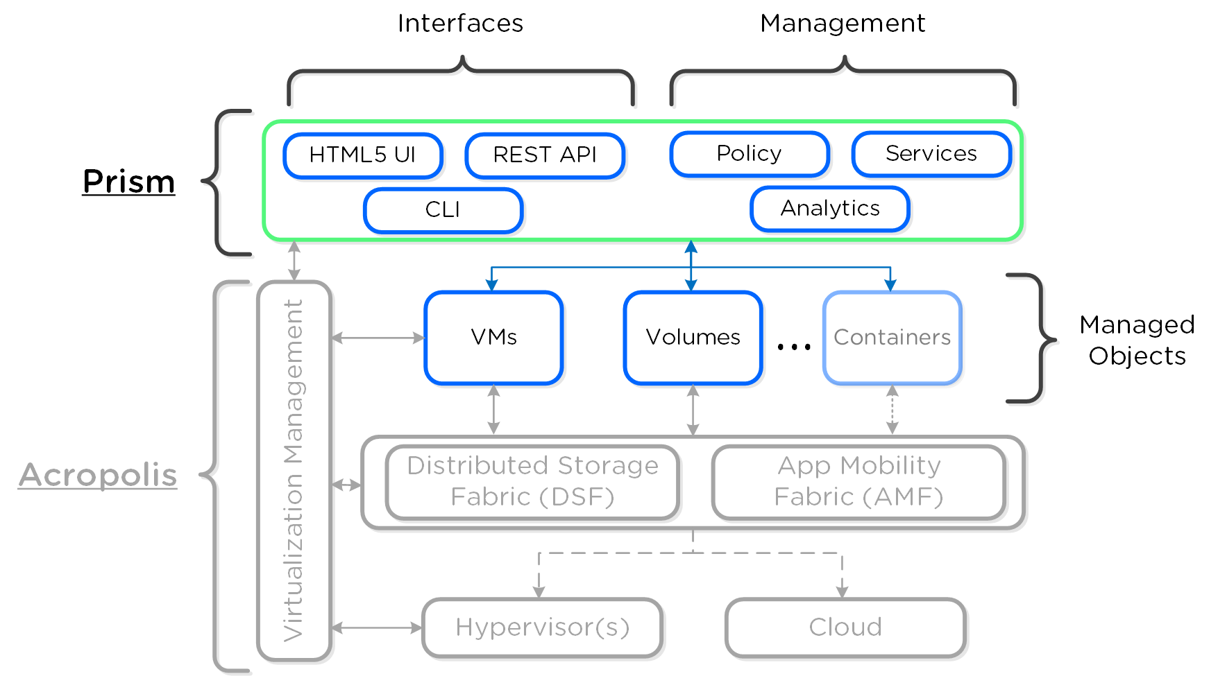
Prism is a distributed resource management platform which allows users to manage and monitor objects and services across their Nutanix environment.
These capabilities are broken down into two key categories:
- Interfaces
- HTML5 UI, REST API, CLI, PowerShell CMDlets, etc.
- Management
- Policy definition and compliance, service design and status, analytics and monitoring
The figure highlights an image illustrating the conceptual nature of Prism as part of the Nutanix platform:
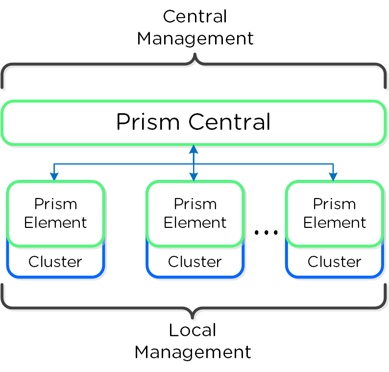
Prism is broken down into two main components:
- Prism Central (PC)
- Multi-cluster manager responsible for managing multiple Acropolis Clusters to provide a single, centralized management interface. Prism Central is an optional software appliance (VM) which can be deployed in addition to the Acropolis Cluster (can run on it).
- 1-to-many cluster manager
- Prism Element (PE)
- Localized cluster manager responsible for local cluster management and operations. Every Acropolis Cluster has Prism Element built-in.
- 1-to-1 cluster manager
The figure shows an image illustrating the conceptual relationship between Prism Central and Prism Element:
Note
Pro tip
For larger or distributed deployments (e.g. more than one cluster or multiple sites) it is recommended to use Prism Central to simplify operations and provide a single management UI for all clusters / sites.
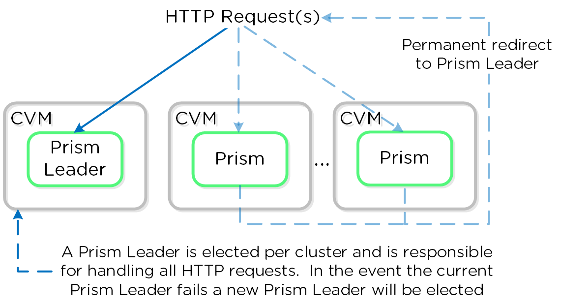
Prism Services
A Prism service runs on every CVM with an elected Prism Leader which is responsible for handling HTTP requests. Similar to other components which have a Master, if the Prism Leader fails, a new one will be elected. When a CVM which is not the Prism Leader gets a HTTP request it will permanently redirect the request to the current Prism Leader using HTTP response status code 301.
Here we show a conceptual view of the Prism services and how HTTP request(s) are handled:
Note
Prism ports
Prism listens on ports 80 and 9440, if HTTP traffic comes in on port 80 it is redirected to HTTPS on port 9440.
When using the cluster external IP (recommended), it will always be hosted by the current Prism Leader. In the event of a Prism Leader failure the cluster IP will be assumed by the newly elected Prism Leader and a gratuitous ARP (gARP) will be used to clean any stale ARP cache entries. In this scenario any time the cluster IP is used to access Prism, no redirection is necessary as that will already be the Prism Leader.
Note
Pro tip
You can determine the current Prism leader by running 'curl localhost:2019/prism/leader' on any CVM.
Navigation
Prism is fairly straight forward and simple to use, however we'll cover some of the main pages and basic usage.
Prism Central (if deployed) can be accessed using the IP address specified during configuration or corresponding DNS entry. Prism Element can be accessed via Prism Central (by clicking on a specific cluster) or by navigating to any Nutanix CVM or cluster IP (preferred).
Once the page has been loaded you will be greeted with the Login page where you will use your Prism or Active Directory credentials to login.
Upon successful login you will be sent to the dashboard page which will provide overview information for managed cluster(s) in Prism Central or the local cluster in Prism Element.
Prism Central and Prism Element will be covered in more detail in the following sections.
Prism Central
Prism Central contains the following main pages:
- Home Page
- Environment wide monitoring dashboard including detailed information on service status, capacity planning, performance, tasks, etc. To get further information on any of them you can click on the item of interest.
- Explore Page
- Management and monitoring of services, cluster, VMs and hosts
- Analysis Page
- Detailed performance analysis for cluster and managed objects with event correlation
- Alerts
- Environment wide alerts
The figure shows a sample Prism Central dashboard where multiple clusters can be monitored / managed:
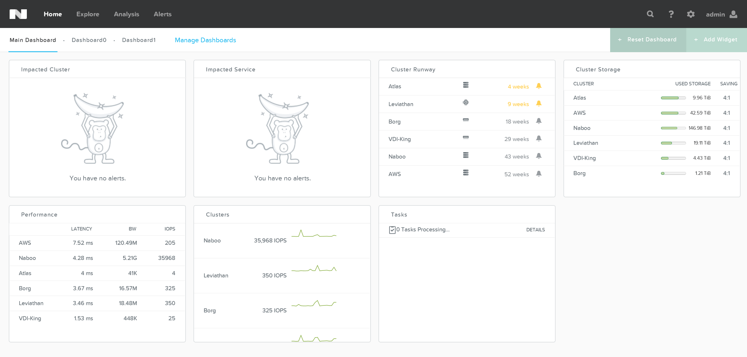
From here you can monitor the overall status of your environment, and dive deeper if there are any alerts or items of interest.
Note
Pro tip
If everything is green, go back to doing something else :)
Prism Element
Prism Element contains the following main pages:
- Home Page
- Local cluster monitoring dashboard including detailed information on alerts, capacity, performance, health, tasks, etc. To get further information on any of them you can click on the item of interest.
- Health Page
- Environment, hardware and managed object health and state information. Includes NCC health check status as well.
- VM Page
- Full VM management, monitoring and CRUD (Acropolis)
- VM monitoring (non-Acropolis)
- Storage Page
- Container management, monitoring and CRUD
- Hardware
- Server, disk and network management, monitoring and health. Includes cluster expansion as well as node and disk removal.
- Data Protection
- DR, Cloud Connect and Metro Availability configuration. Management of PD objects, snapshots, replication and restore.
- Analysis
- Detailed performance analysis for cluster and managed objects with event correlation
- Alerts
- Local cluster and environment alerts
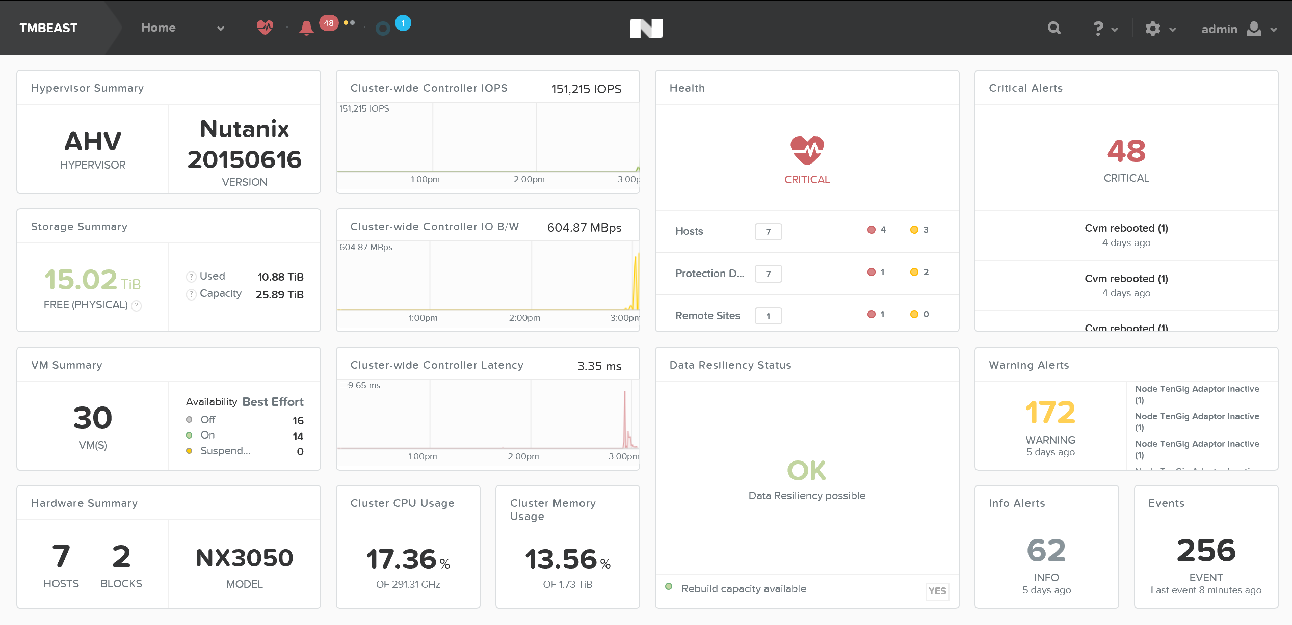
The home page will provide detailed information on alerts, service status, capacity, performance, tasks, and much more. To get further information on any of them you can click on the item of interest.
The figure shows a sample Prism Element dashboard where local cluster details are displayed:
Note
Keyboard Shortcuts
Accessibility and ease of use is a very critical construct in Prism. To simplify things for the end-user a set of shortcuts have been added to allow users to do everything from their keyboard.
The following characterizes some of the key shortcuts:
Change view (page context aware):
- O - Overview View
- D - Diagram View
- T - Table View
Activities and Events:
- A - Alerts
- P - Tasks
Drop down and Menus (Navigate selection using arrow keys):
- M - Menu drop-down
- S - Settings (gear icon)
- F - Search bar
- U - User drop down
- H - Help
Usage and Troubleshooting
In the following sections we'll cover some of the typical Prism uses as well as some common troubleshooting scenarios.
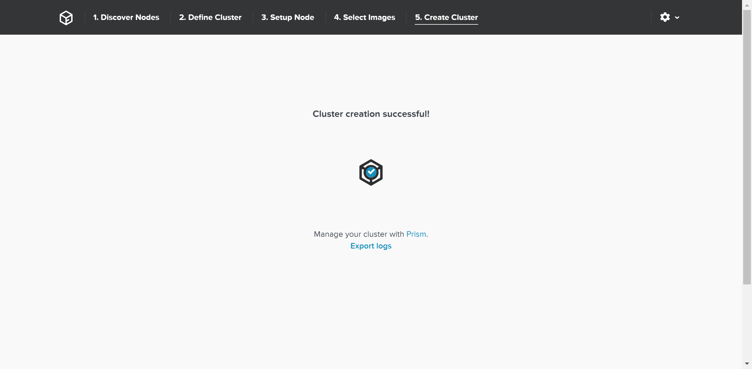
Nutanix Software Upgrade
Performing a Nutanix software upgrade is a very simple and non-disruptive process.
To begin, start by logging into Prism and clicking on the gear icon on the top right (settings) or by pressing 'S' and selecting 'Upgrade Software':
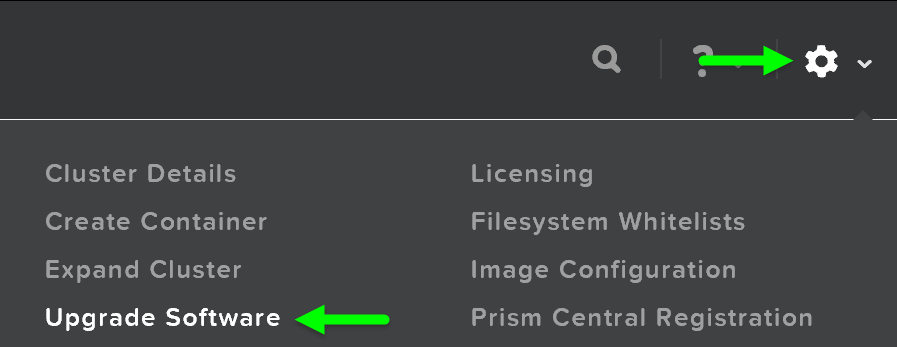
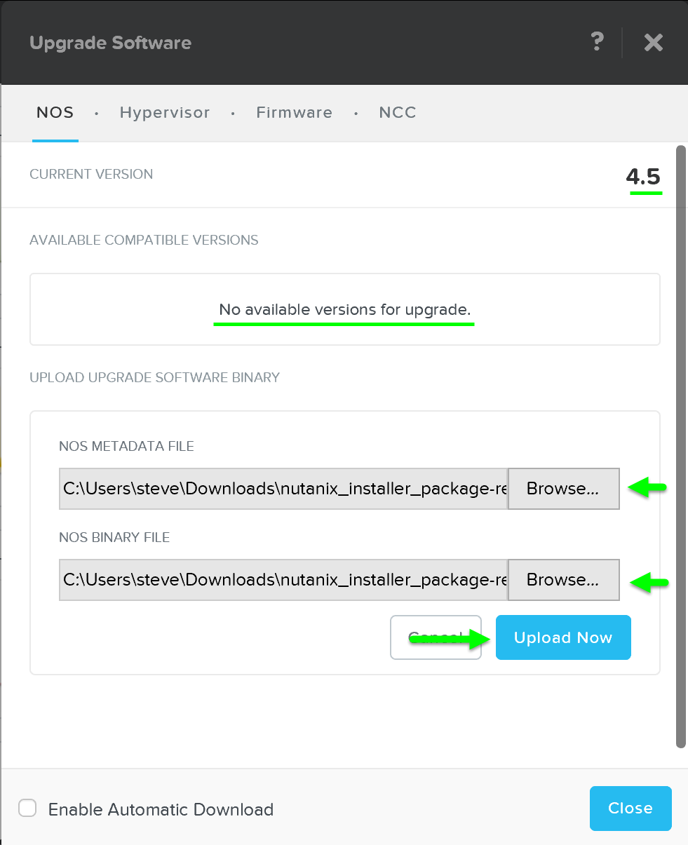
This will launch the 'Upgrade Software' dialog box and will show your current software version and if there are any upgrade versions available. It is also possible to manually upload a NOS binary file.
You can then download the upgrade version from the cloud or upload the version manually:
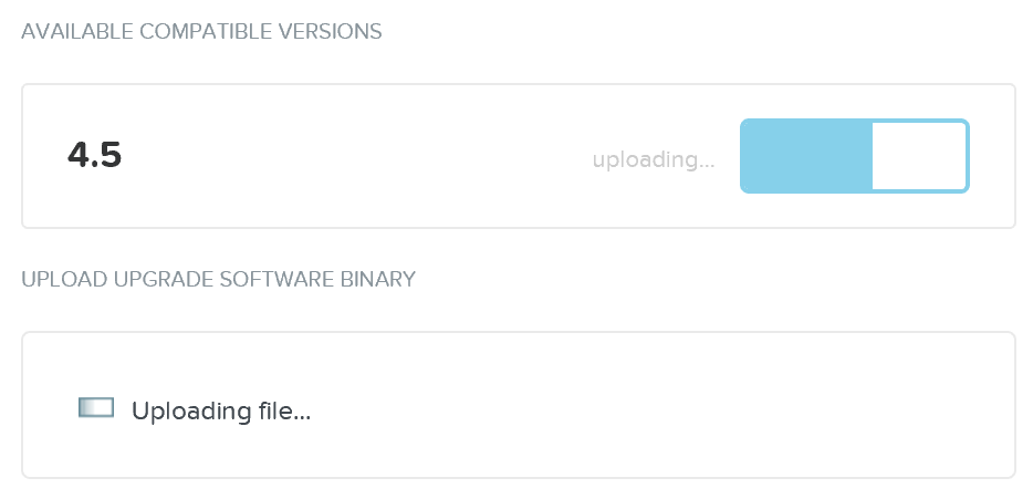
It will then upload the upgrade software onto the Nutanix CVMs:
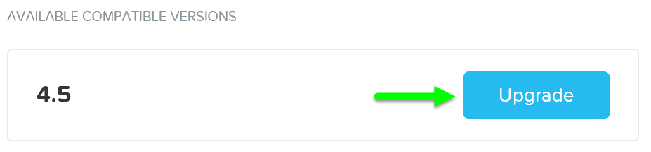
After the software is loaded click on 'Upgrade' to start the upgrade process:
You'll then be prompted with a confirmation box:

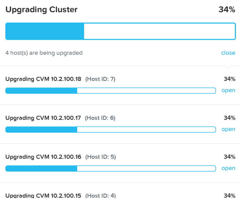
The upgrade will start with pre-upgrade checks then start upgrading the software in a rolling manner:
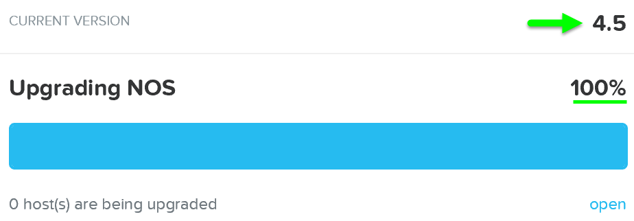
Once the upgrade is complete you'll see an updated status and have access to all of the new features:
Note
Note
Your Prism session will briefly disconnect during the upgrade when the current Prism Leader is upgraded. All VMs and services running remain unaffected.
Hypervisor Upgrade
Similar to Nutanix software upgrades, hypervisor upgrades can be fully automated in a rolling manner via Prism.
To begin follow the similar steps above to launch the 'Upgrade Software' dialogue box and select 'Hypervisor'.
You can then download the hypervisor upgrade version from the cloud or upload the version manually:
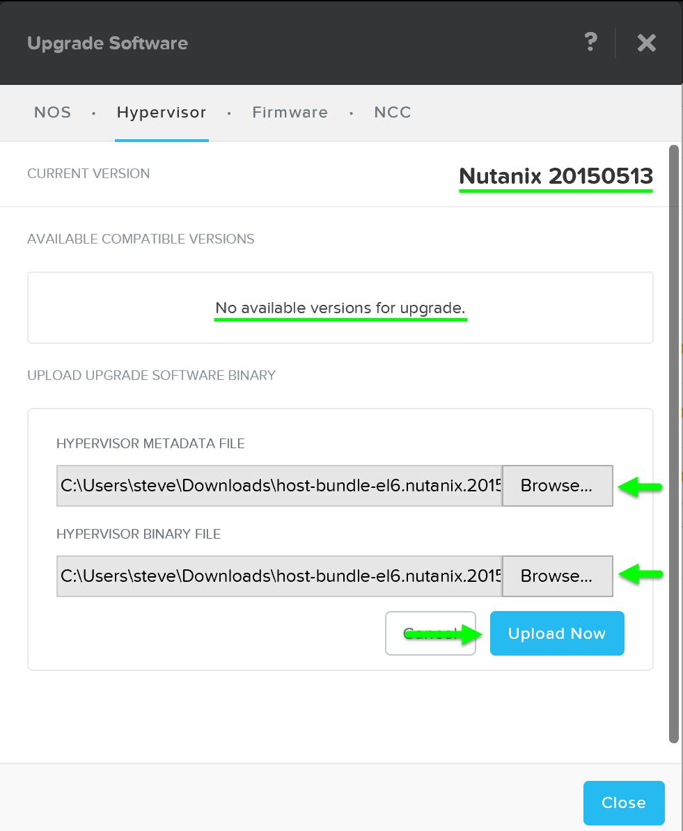
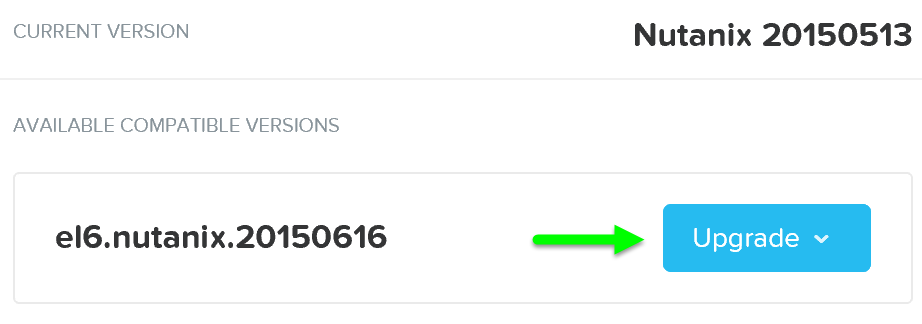
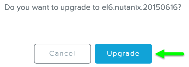
It will then load the upgrade software onto the Hypervisors. After the software is loaded click on 'Upgrade' to start the upgrade process:
You'll then be prompted with a confirmation box:
The system will then go through host pre-upgrade checks and upload the hypervisor upgrade to the cluster:
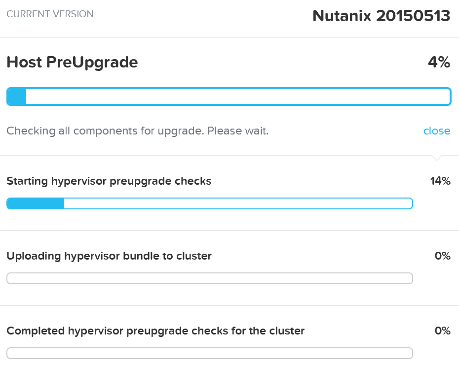
Once the pre-upgrade checks are complete the rolling hypervisor upgrade will then proceed:
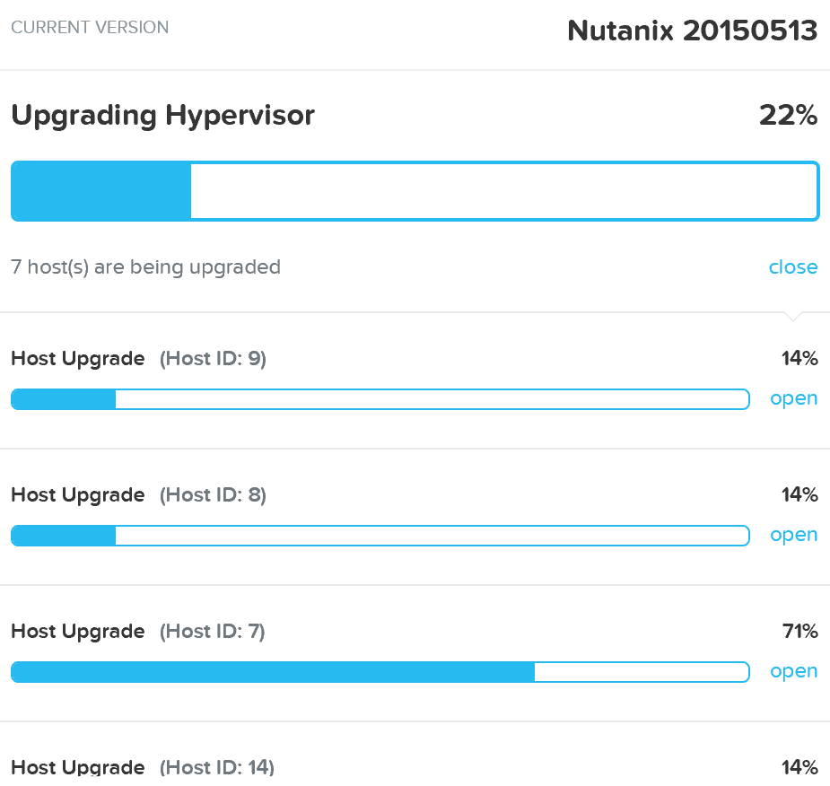
Similar to the rolling nature of the Nutanix software upgrades, each host will be upgraded in a rolling manner with zero impact to running VMs. VMs will be live-migrated off the current host, the host will be upgraded, and then rebooted. This process will iterate through each host until all hosts in the cluster are upgraded.
Note
Pro tip
You can also get cluster wide upgrade status from any Nutanix CVM by running 'host_upgrade --status'. The detailed per host status is logged to ~/data/logs/host_upgrade.out on each CVM.
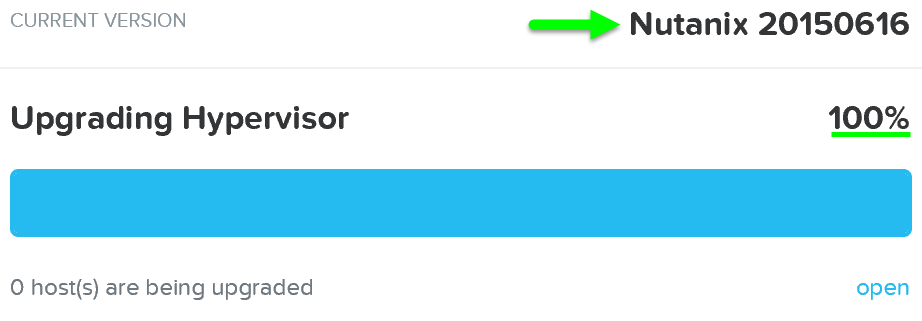
Once the upgrade is complete you'll see an updated status and have access to all of the new features:
Cluster Expansion (add node)
The ability to dynamically scale the Acropolis cluster is core to its functionality. To scale an Acropolis cluster, rack / stack / cable the nodes and power them on. Once the nodes are powered up they will be discoverable by the current cluster using mDNS.
The figure shows an example 7 node cluster with 1 node which has been discovered:
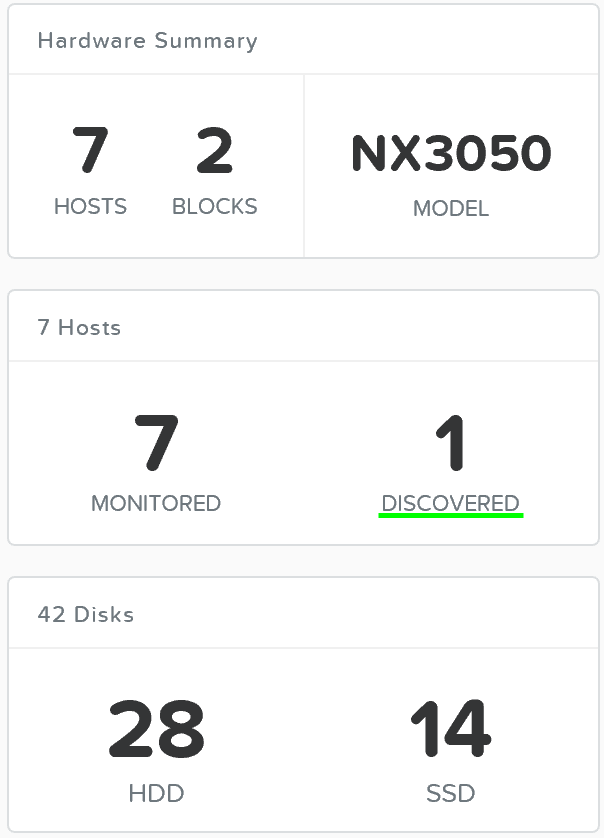
Multiple nodes can be discovered and added to the cluster concurrently.
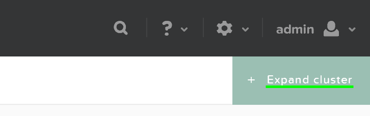
Once the nodes have been discovered you can begin the expansion by clicking 'Expand Cluster' on the upper right hand corner of the 'Hardware' page:
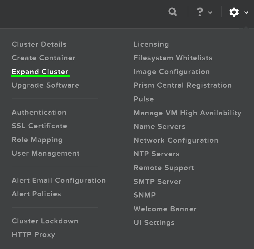
You can also begin the cluster expansion process from any page by clicking on the gear icon:
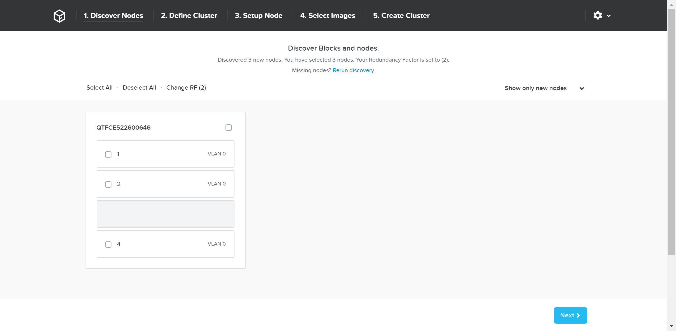
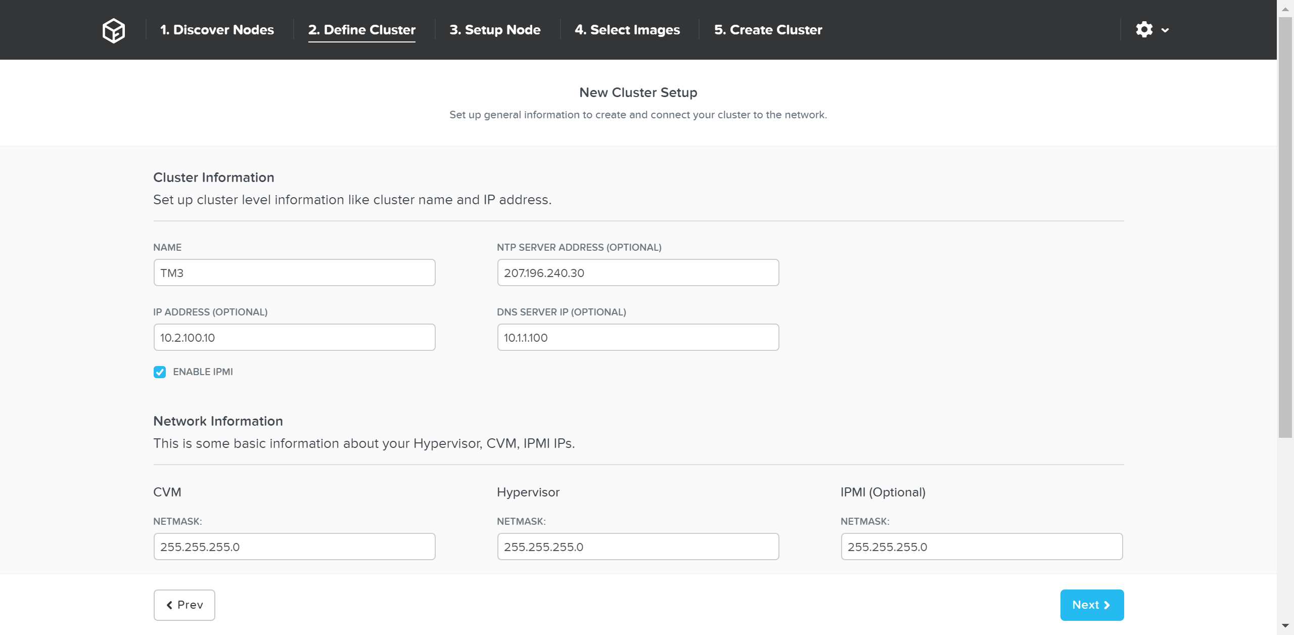
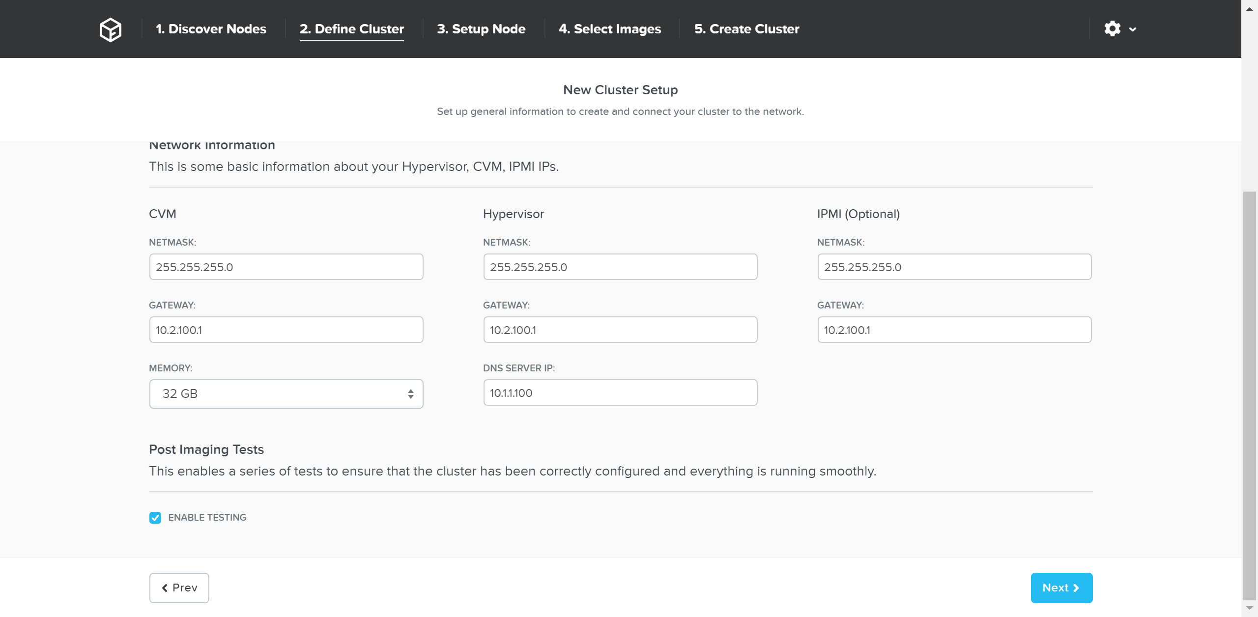
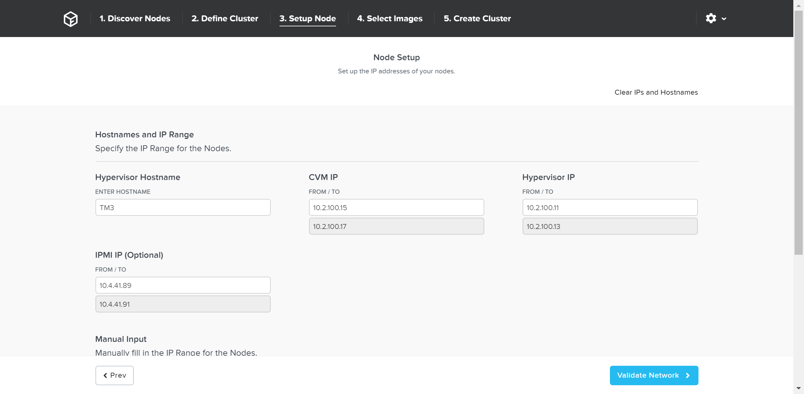
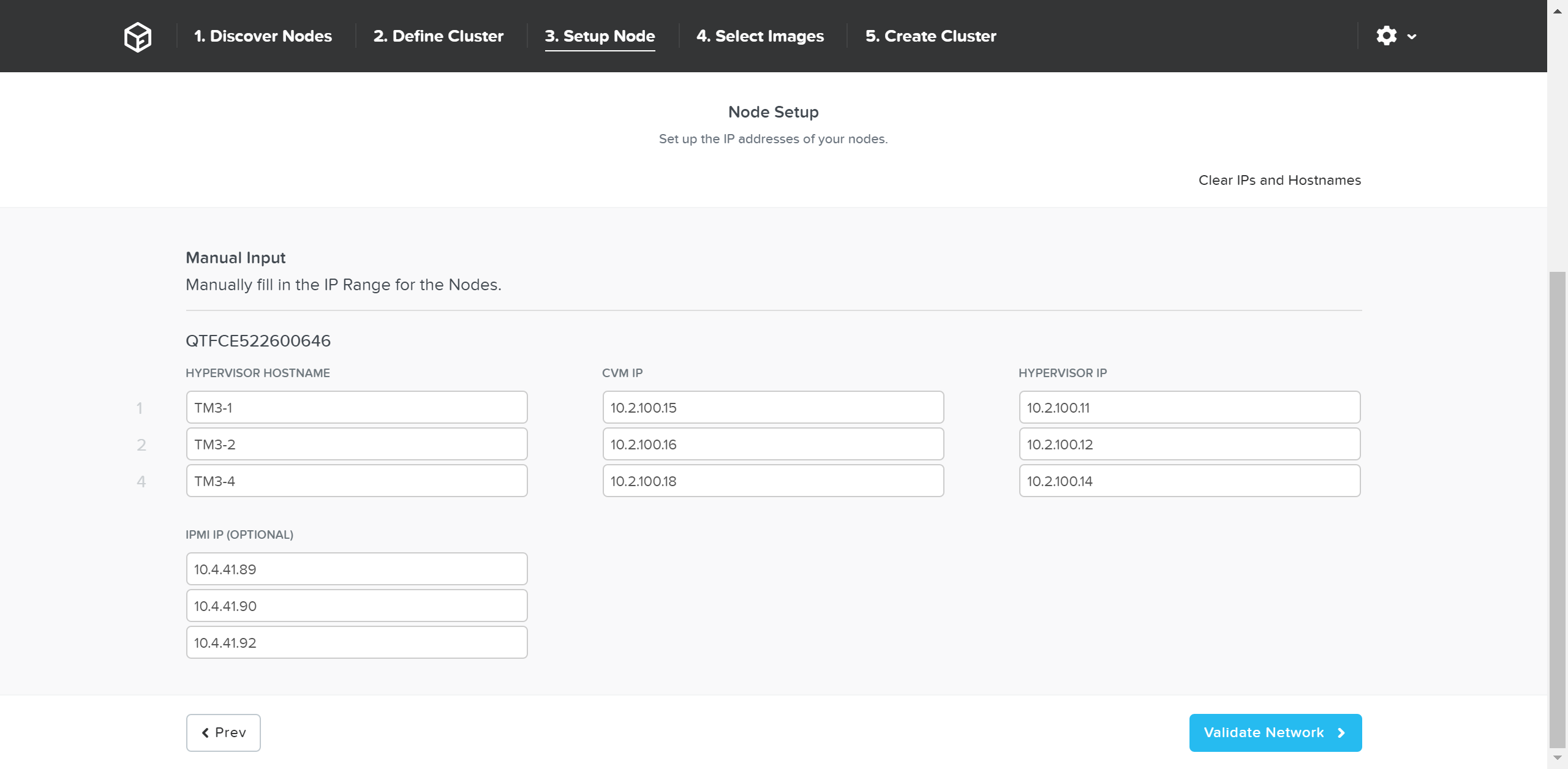
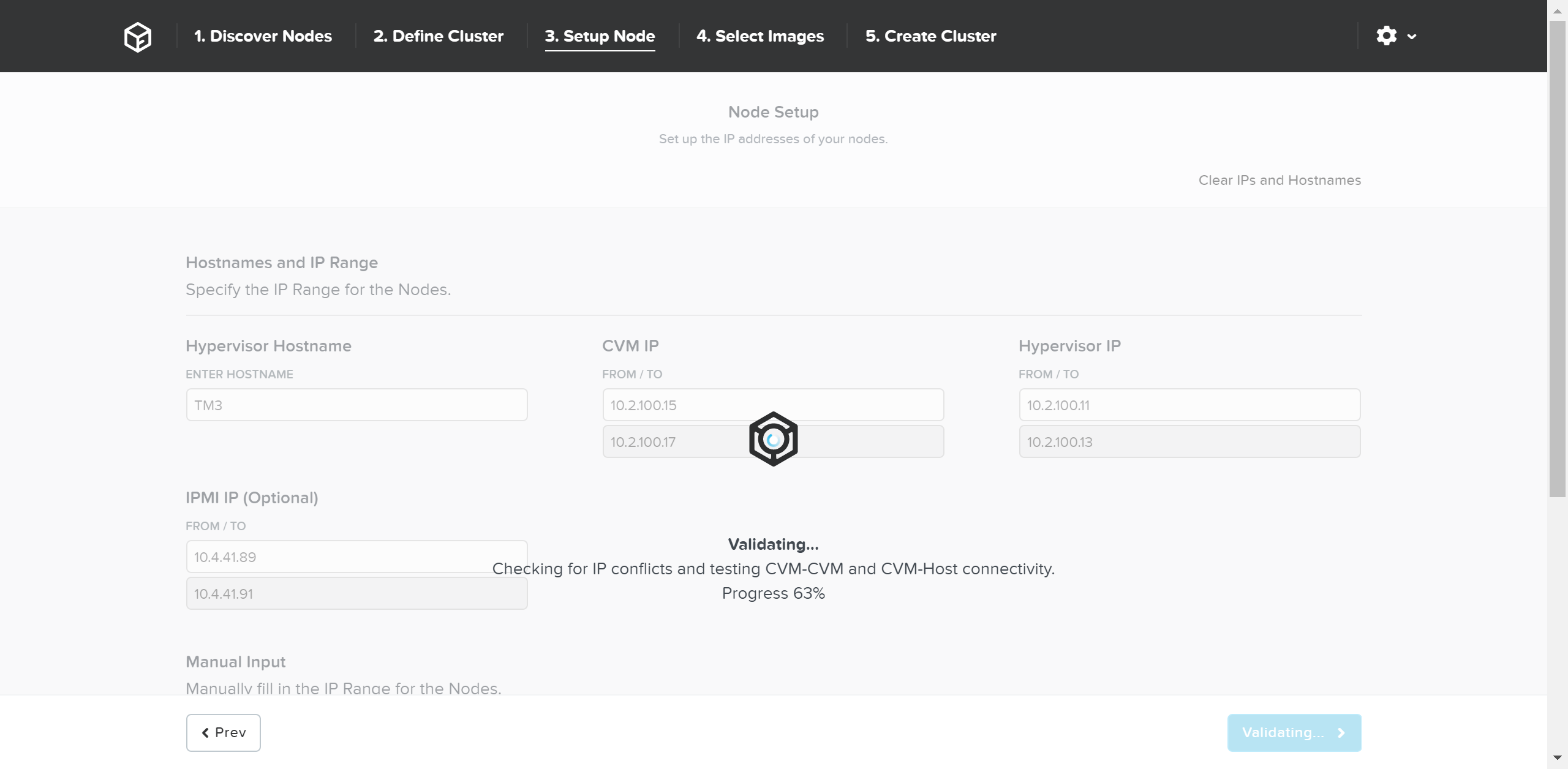
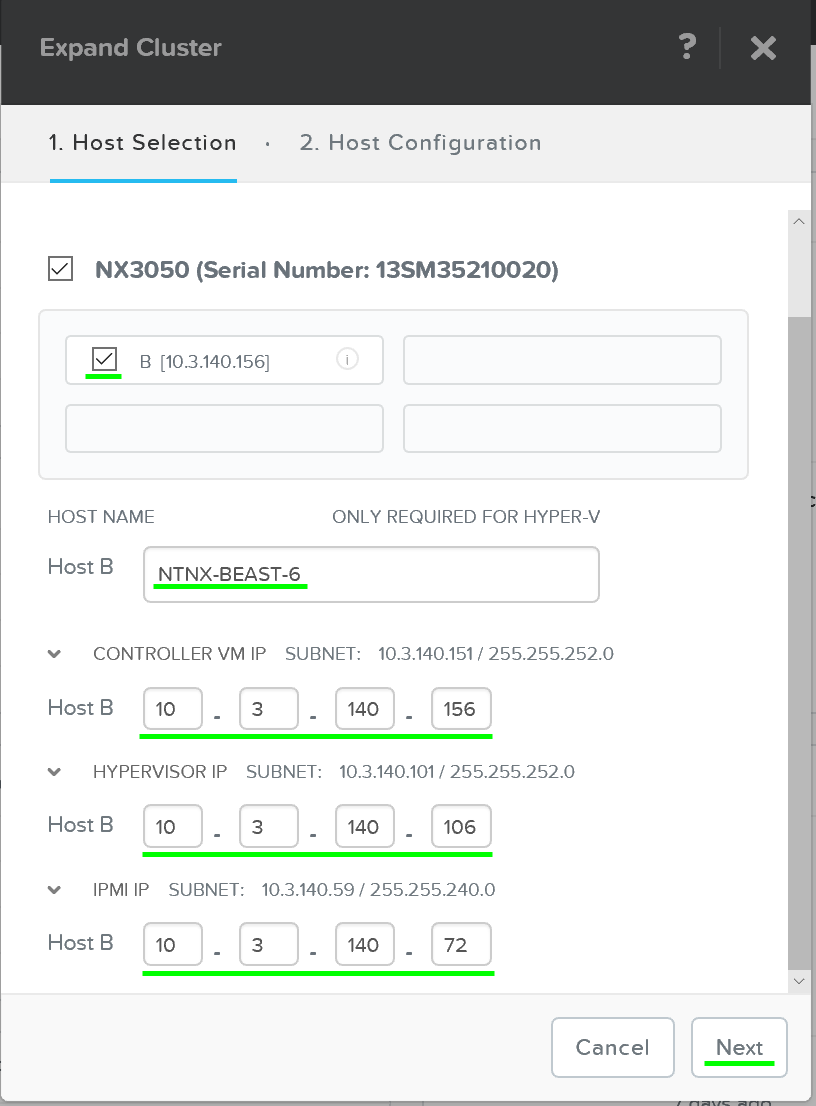
This launches the expand cluster menu where you can select the node(s) to add and specify IP addresses for the components:
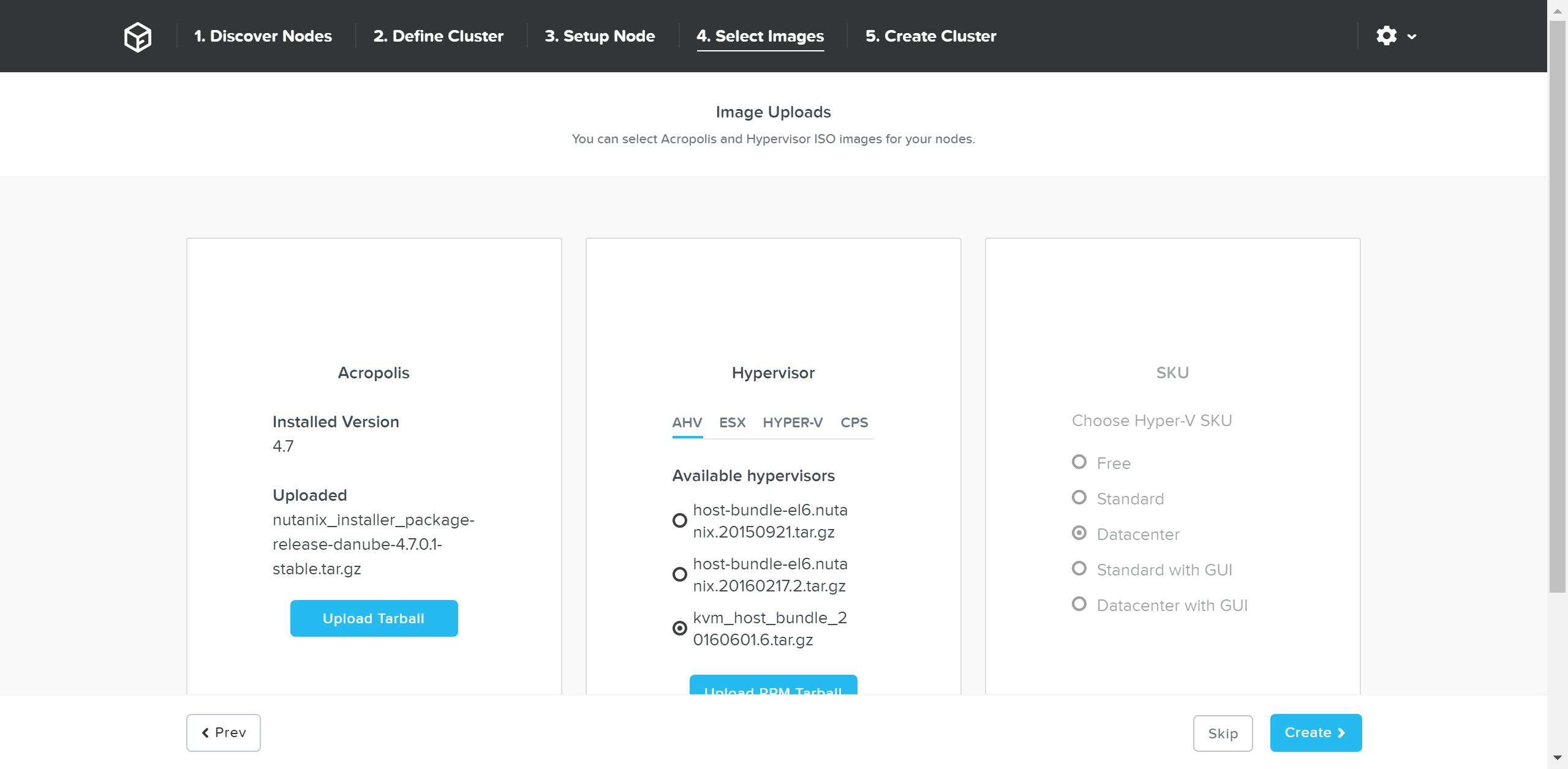
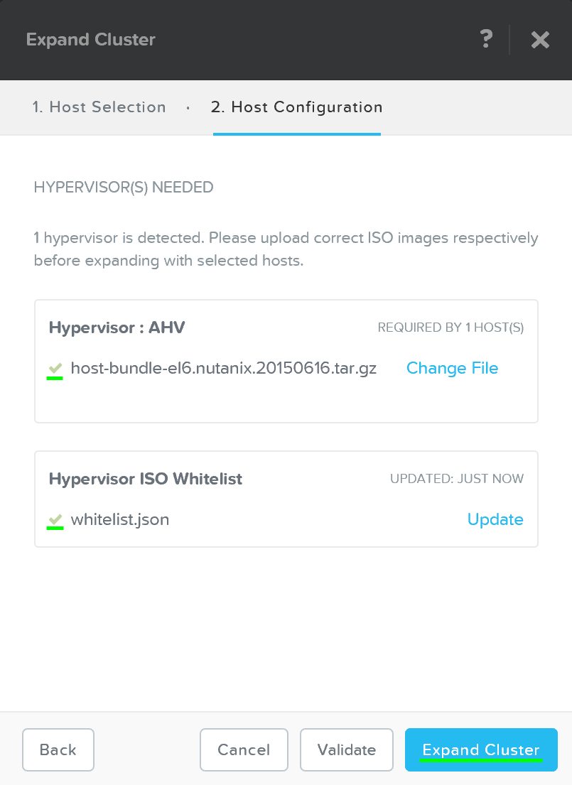
After the hosts have been selected you'll be prompted to upload a hypervisor image which will be used to image the nodes being added. For AHV or cases where the image already exists in the Foundation installer store, no upload is necessry.
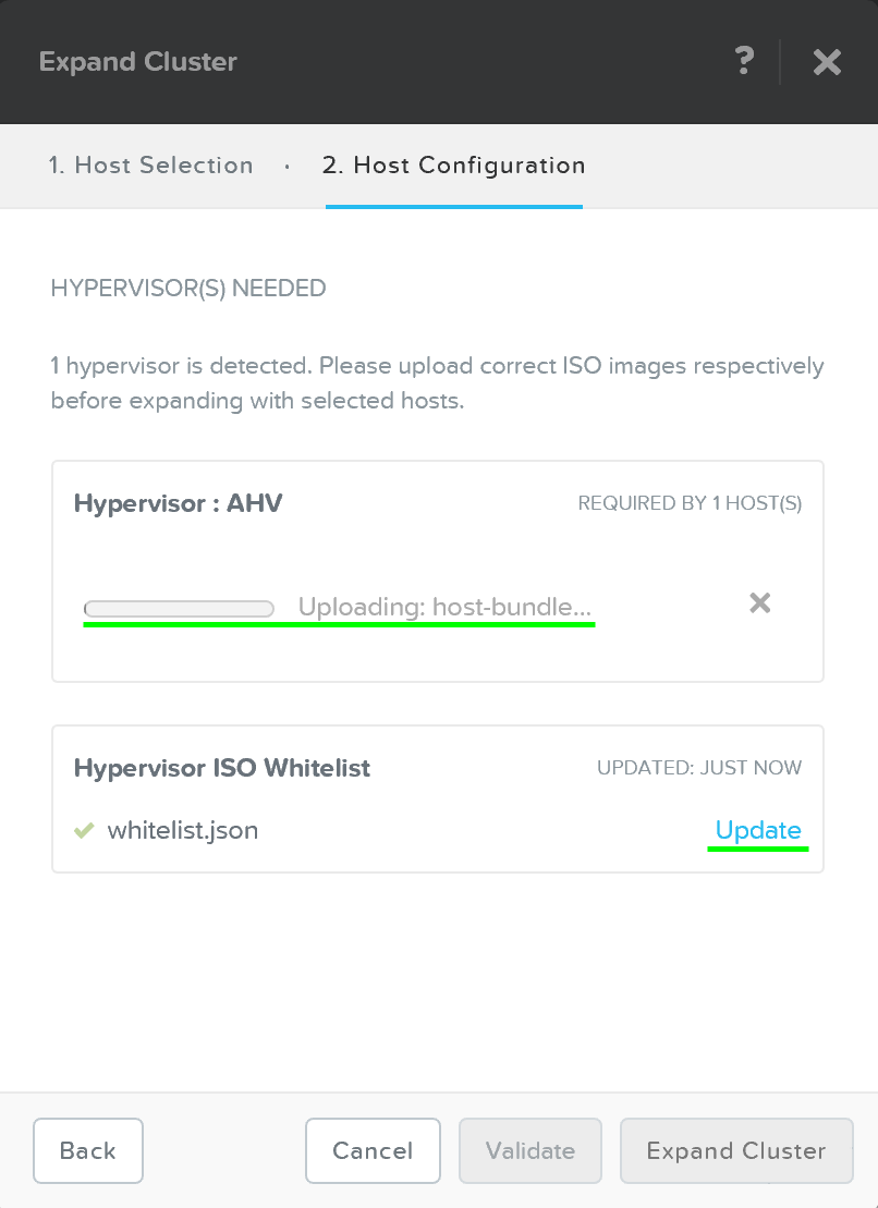
After the upload is completed you can click on 'Expand Cluster' to begin the imaging and expansion process:
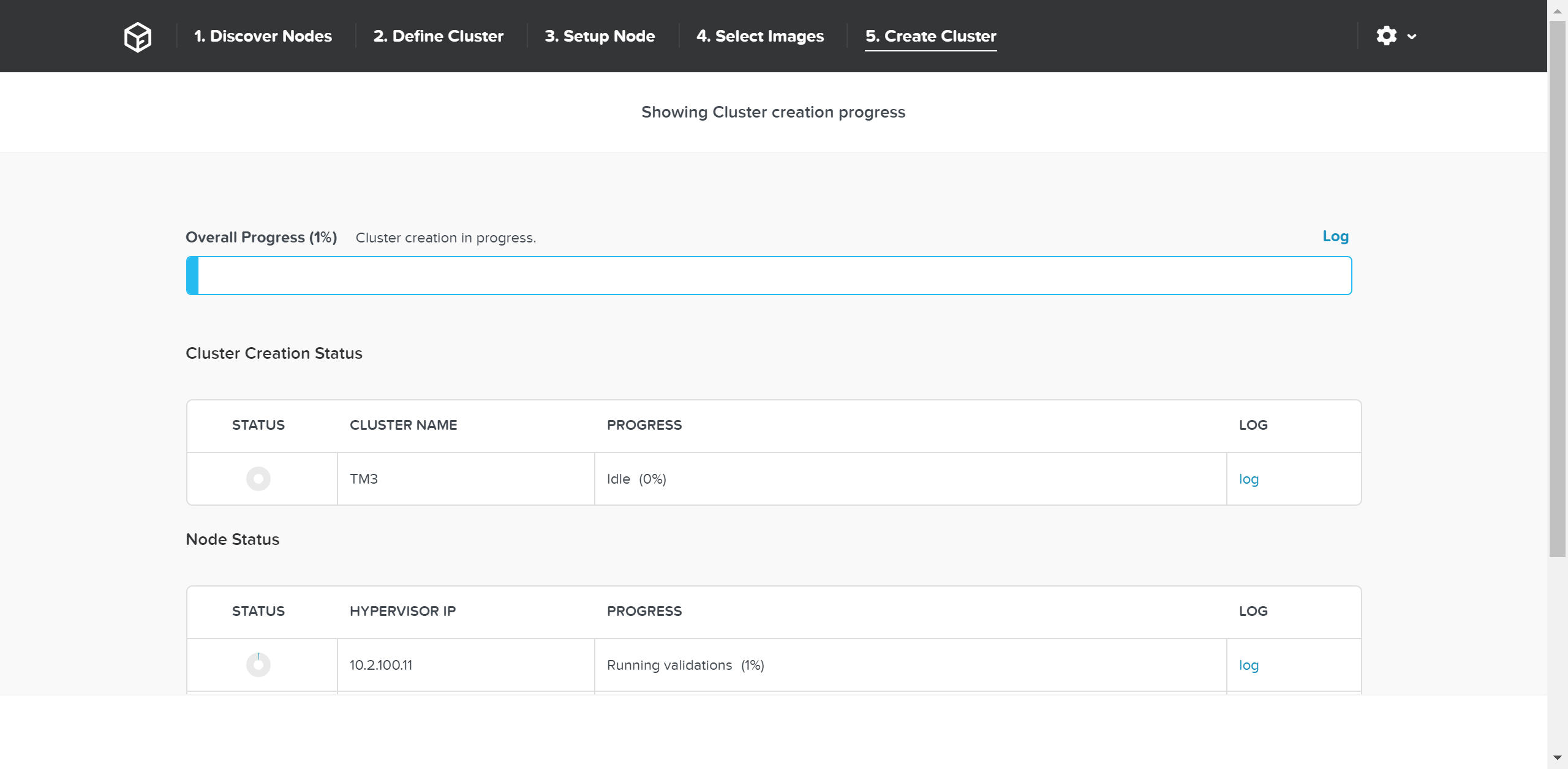
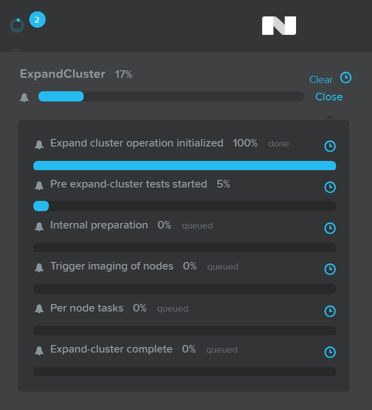
The job will then be submitted and the corresponding task item will appear:

Detailed tasks status can be viewed by expanding the task(s):
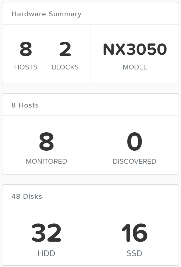
After the imaging and add node process has been completed you'll see the updated cluster size and resources:
I/O Metrics
Identification of bottlenecks is a critical piece of the performance troubleshooting process. In order to aid in this process, Nutanix has introduced a new 'I/O Metrics' section to the VM page.
Latency is dependent on multitude of variables (queue depth, I/O size, system conditions, netowrk speed, etc.). This page aims to offer insight on the I/O size, latency, source, and patterns.
To use the new section, go to the 'VM' page and select a desired VM from the table. Here we can see high level usage metrics:

The 'I/O Metrics' tab can be found in the section below the table:

Upon selecting the 'I/O Metrics' tab a detailed view will be shown. We will break this page down and how to use it in the following.
The first view is the 'Avg I/O Latency' section that shows average R/W latency for the past three hours. By default the latest reported values are shown with the corresponding detailed metrics below for that point in time.
You can also mouse over the plot to see the historical latency values and click on a time of the plot to view the detailed metrics below.
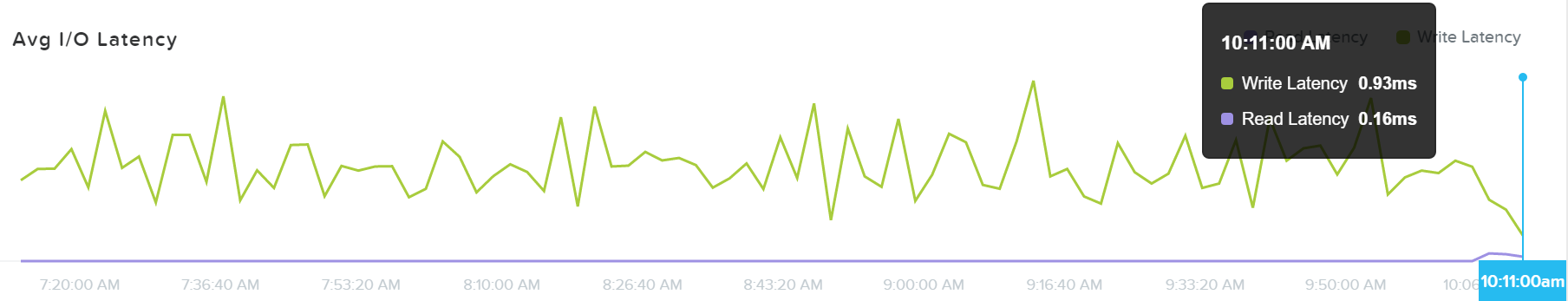
This can be useful when a sudden spike is seen. If you see a spike and want to investigate further, click on the spike and evaluate the details below.
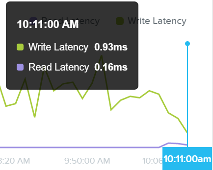
If latency is all good, no need to dig any further.
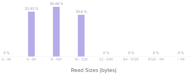
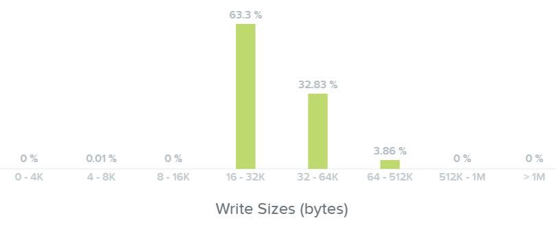
The next section shows a historgram of I/O sizes for read and write I/Os:
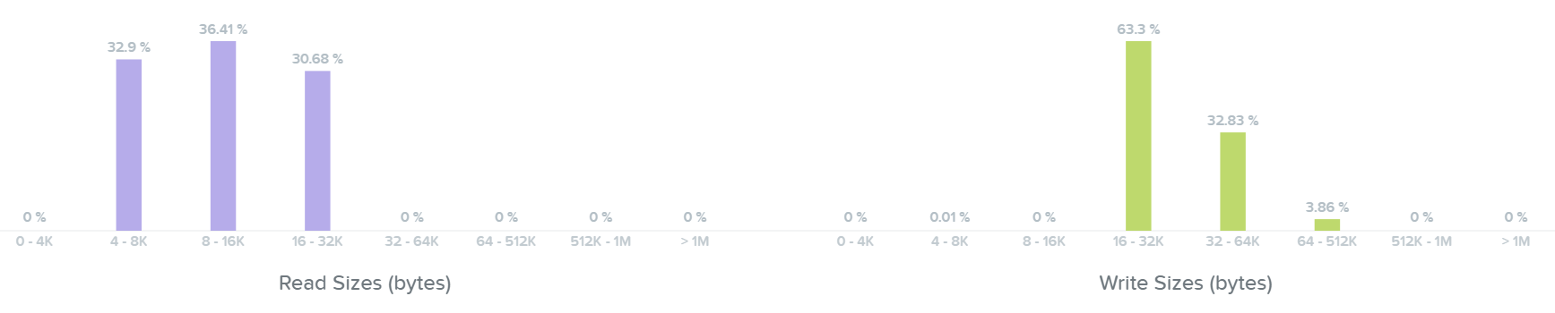
Here we can see our read I/Os range from 4K to 32K in size:
Here we can see our write I/Os range from 16K to 64K with some up to 512K in size:
Note
Pro tip
If you see a spike in latency the first thing to check is the I/O size. Larger I/Os (64K up to 1MB) will typically see higher latencies than smaller I/Os (4K to 32K).
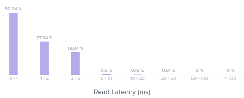
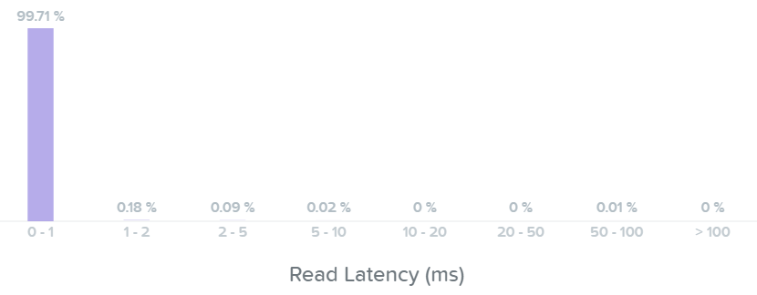
The next section shows a historgram of I/O latencies for read and write I/Os:
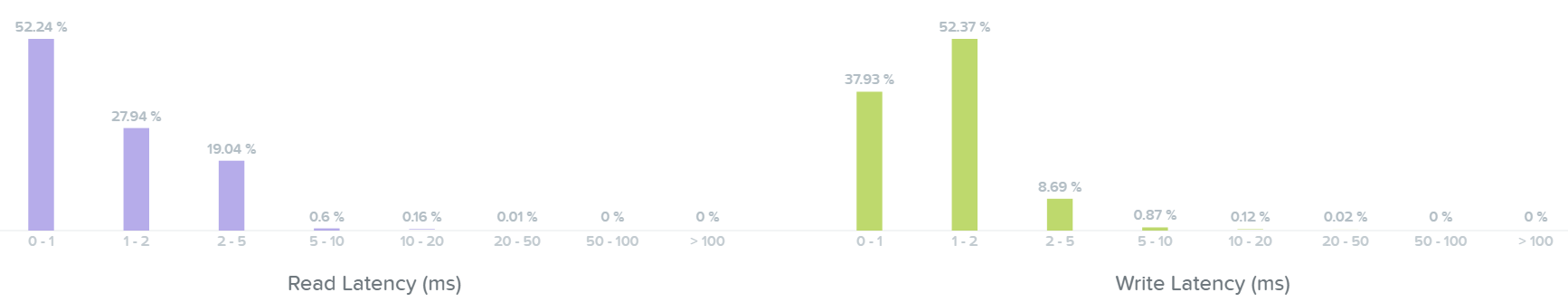
Looking at the read latency histogram we can see the majority of read I/Os are sub-ms (<1ms) with some up to 2-5ms.
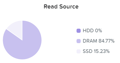
Taking a look below at the 'Read Source' we can see most I/Os are being served from the SSD tier:
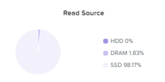
As data is read it will be pulled in to the Unified Cache (DRAM+SSD) realtime (Check the 'I/O Path and Cache' section to learn more). Here we can see the data has been pulled into the cache and is now being served from DRAM:
We can now see basically all of our read I/Os are seeing sub-ms (<1ms) latency:
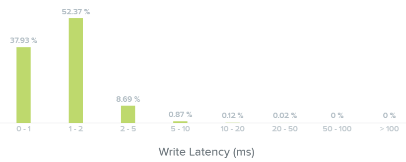
Here we can see the majority of our write I/O are seeing <1-2ms latency:
Note
Pro tip
If you see a spike in read latency and the I/O sizes aren't large, check where the read I/Os are being served from. Any initial read from HDD will see higher latency than the DRAM cache; however, once it is in the cache all subsequent reads will hit DRAM and see an improvement in latency.
The last section shows the I/O patterns and how much is random vs. sequential:
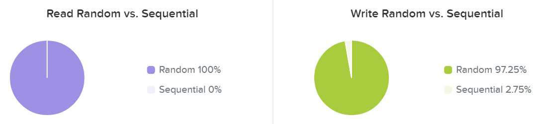
Typically I/O patterns will vary by application or workload (e.g. VDI is mainly random, whereas Hadoop would primarily be sequential). Other workloads will be a mix of both. For example, a database might be random on inserts or some queries, however sequential during ETL.
Capacity Planning
To get detailed capacity planning details you can click on a specific cluster under the 'cluster runway' section in Prism Central to get more details:
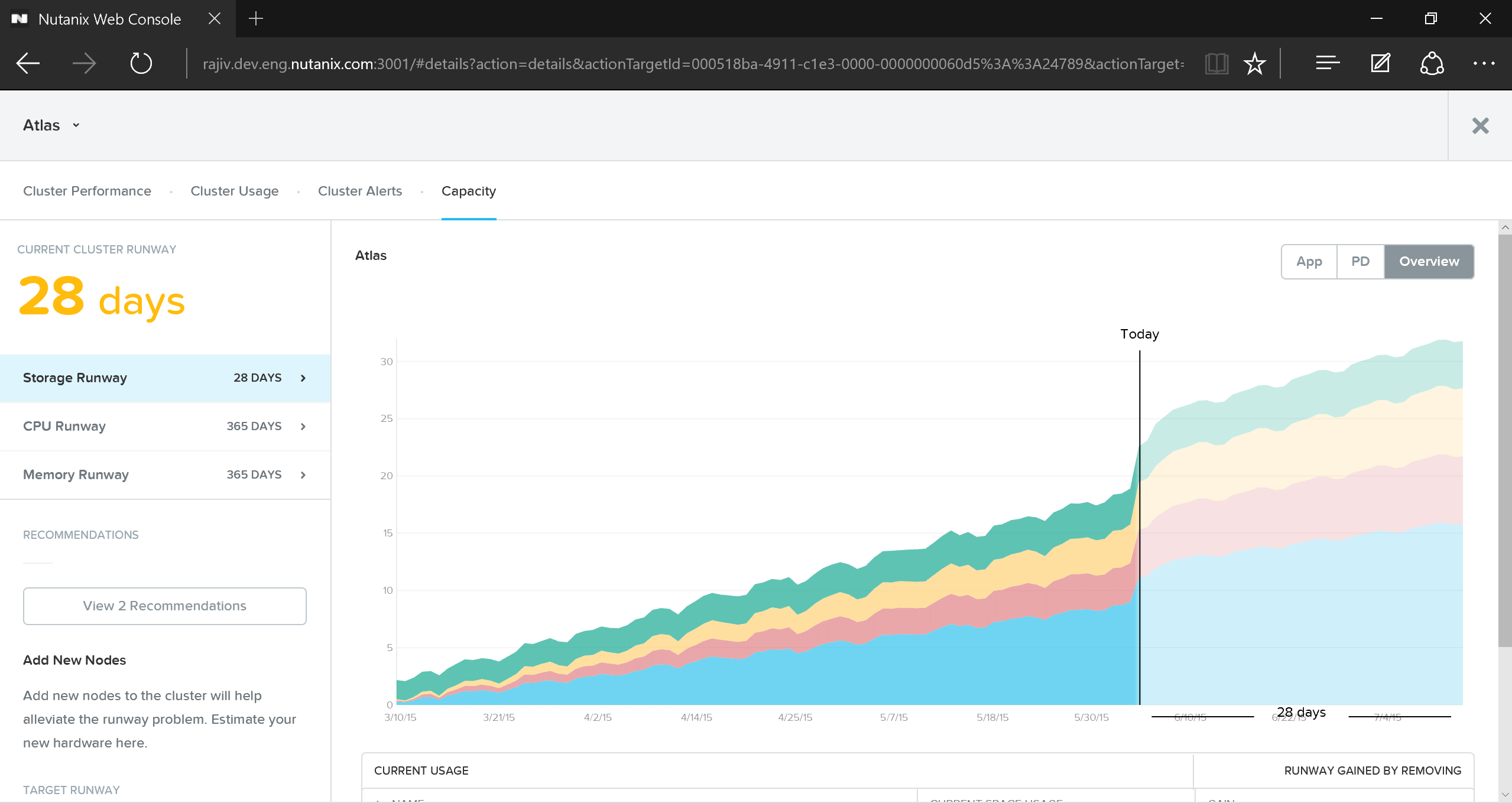
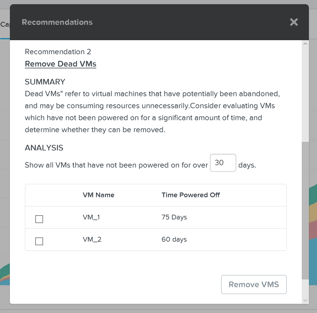
This view provides detailed information on cluster runway and identifies the most constrained resource (limiting resource). You can also get detailed information on what the top consumers are as well as some potential options to clean up additional capacity or ideal node types for cluster expansion.
The HTML5 UI is a key part to Prism to provide a simple, easy to use management interface. However, another core ability are the APIs which are available for automation. All functionality exposed through the Prism UI is also exposed through a full set of REST APIs to allow for the ability to programmatically interface with the Nutanix platform. This allow customers and partners to enable automation, 3rd-party tools, or even create their own UI.
The following section covers these interfaces and provides some example usage.
APIs and Interfaces
Core to any dynamic or “software-defined” environment, Nutanix provides a vast array of interfaces allowing for simple programmability and interfacing. Here are the main interfaces:
- REST API
- CLI - ACLI & NCLI
- Scripting interfaces
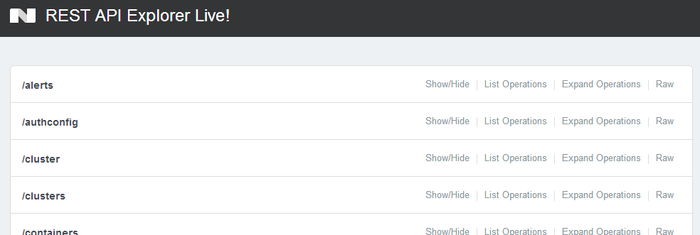
Core to this is the REST API which exposes every capability and data point of the Prism UI and allows for orchestration or automation tools to easily drive Nutanix action. This enables tools like Saltstack, Puppet, vRealize Operations, System Center Orchestrator, Ansible, etc. to easily create custom workflows for Nutanix. Also, this means that any third-party developer could create their own custom UI and pull in Nutanix data via REST.
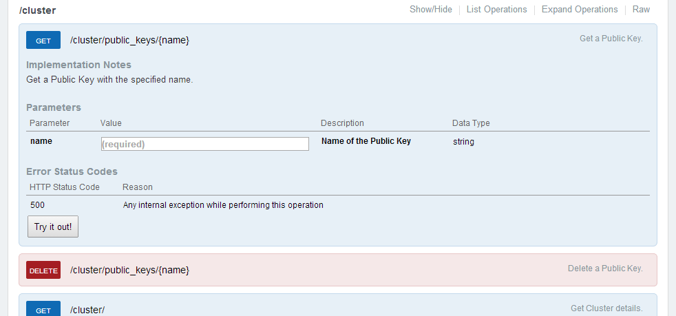
The following figure shows a small snippet of the Nutanix REST API explorer which allows developers to interact with the API and see expected data formats:
Operations can be expanded to display details and examples of the REST call:
Note
API Authentication Scheme(s)
As of 4.5.x basic authentication over HTTPS is leveraged for client and HTTP call authentication.
ACLI
The Acropolis CLI (ACLI) is the CLI for managing the Acropolis portion of the Nutanix product. These capabilities were enabled in releases after 4.1.2.
NOTE: All of these actions can be performed via the HTML5 GUI and REST API. I just use these commands as part of my scripting to automate tasks.
Enter ACLI shell
Description: Enter ACLI shell (run from any CVM)
Acli
OR
Description: Execute ACLI command via Linux shell
ACLI <Command>
Output ACLI response in json format
Description: Lists Acropolis nodes in the cluster.
Acli –o json
List hosts
Description: Lists Acropolis nodes in the cluster.
host.list
Create network
Description: Create network based on VLAN
net.create <TYPE>.<ID>[.<VSWITCH>] ip_config=<A.B.C.D>/<NN>
Example: net.create vlan.133 ip_config=10.1.1.1/24
List network(s)
Description: List networks
net.list
Create DHCP scope
Description: Create dhcp scope
net.add_dhcp_pool <NET NAME> start=<START IP A.B.C.D> end=<END IP W.X.Y.Z>
Note: .254 is reserved and used by the Acropolis DHCP server if an address for the Acropolis DHCP server wasn’t set during network creation
Example: net.add_dhcp_pool vlan.100 start=10.1.1.100 end=10.1.1.200
Get an existing networks details
Description: Get a network's properties
net.get <NET NAME>
Example: net.get vlan.133
Get an existing networks details
Description: Get a network's VMs and details including VM name / UUID, MAC address and IP
net.list_vms <NET NAME>
Example: net.list_vms vlan.133
Configure DHCP DNS servers for network
Description: Set DHCP DNS
net.update_dhcp_dns <NET NAME> servers=<COMMA SEPARATED DNS IPs> domains=<COMMA SEPARATED DOMAINS>
Example: net.set_dhcp_dns vlan.100 servers=10.1.1.1,10.1.1.2 domains=splab.com
Create Virtual Machine
Description: Create VM
vm.create <COMMA SEPARATED VM NAMES> memory=<NUM MEM MB> num_vcpus=<NUM VCPU> num_cores_per_vcpu=<NUM CORES> ha_priority=<PRIORITY INT>
Example: vm.create testVM memory=2G num_vcpus=2
Bulk Create Virtual Machine
Description: Create bulk VM
vm.create <CLONE PREFIX>[<STARTING INT>..<END INT>] memory=<NUM MEM MB> num_vcpus=<NUM VCPU> num_cores_per_vcpu=<NUM CORES> ha_priority=<PRIORITY INT>
Example: vm.create testVM[000..999] memory=2G num_vcpus=2
Clone VM from existing
Description: Create clone of existing VM
vm.clone <CLONE NAME(S)> clone_from_vm=<SOURCE VM NAME>
Example: vm.clone testClone clone_from_vm=MYBASEVM
Bulk Clone VM from existing
Description: Create bulk clones of existing VM
vm.clone <CLONE PREFIX>[<STARTING INT>..<END INT>] clone_from_vm=<SOURCE VM NAME>
Example: vm.clone testClone[001..999] clone_from_vm=MYBASEVM
Create disk and add to VM
# Description: Create disk for OS
vm.disk_create <VM NAME> create_size=<Size and qualifier, e.g. 500G> container=<CONTAINER NAME>
class="codetext"Example: vm.disk_create testVM create_size=500G container=default
Add NIC to VM
Description: Create and add NIC
vm.nic_create <VM NAME> network=<NETWORK NAME> model=<MODEL>
Example: vm.nic_create testVM network=vlan.100
Set VM’s boot device to disk
Description: Set a VM boot device
Set to boot form specific disk id
vm.update_boot_device <VM NAME> disk_addr=<DISK BUS>
Example: vm.update_boot_device testVM disk_addr=scsi.0
Set VM’s boot device to CDrom
Set to boot from CDrom
vm.update_boot_device <VM NAME> disk_addr=<CDROM BUS>
Example: vm.update_boot_device testVM disk_addr=ide.0
Mount ISO to CDrom
Description: Mount ISO to VM cdrom
Steps:
1. Upload ISOs to container
2. Enable whitelist for client IPs
3. Upload ISOs to share
Create CDrom with ISO
vm.disk_create <VM NAME> clone_nfs_file=<PATH TO ISO> cdrom=true
Example: vm.disk_create testVM clone_nfs_file=/default/ISOs/myfile.iso cdrom=true
If a CDrom is already created just mount it
vm.disk_update <VM NAME> <CDROM BUS> clone_nfs_file<PATH TO ISO>
Example: vm.disk_update atestVM1 ide.0 clone_nfs_file=/default/ISOs/myfile.iso
Detach ISO from CDrom
Description: Remove ISO from CDrom
vm.disk_update <VM NAME> <CDROM BUS> empty=true
Power on VM(s)
Description: Power on VM(s)
vm.on <VM NAME(S)>
Example: vm.on testVM
Power on all VMs
Example: vm.on *
Power on all VMs matching a prefix
Example: vm.on testVM*
Power on range of VMs
Example: vm.on testVM[0-9][0-9]
NCLI
NOTE: All of these actions can be performed via the HTML5 GUI and REST API. I just use these commands as part of my scripting to automate tasks.
Add subnet to NFS whitelist
Description: Adds a particular subnet to the NFS whitelist
ncli cluster add-to-nfs-whitelist ip-subnet-masks=10.2.0.0/255.255.0.0
Display Nutanix Version
Description: Displays the current version of the Nutanix software
ncli cluster version
Display hidden NCLI options
Description: Displays the hidden ncli commands/options
ncli helpsys listall hidden=true [detailed=false|true]
List Storage Pools
Description: Displays the existing storage pools
ncli sp ls
List containers
Description: Displays the existing containers
ncli ctr ls
Create container
Description: Creates a new container
ncli ctr create name=<NAME> sp-name=<SP NAME>
List VMs
Description: Displays the existing VMs
ncli vm ls
List public keys
Description: Displays the existing public keys
ncli cluster list-public-keys
Add public key
Description: Adds a public key for cluster access
SCP public key to CVM
Add public key to cluster
ncli cluster add-public-key name=myPK file-path=~/mykey.pub
Remove public key
Description: Removes a public key for cluster access
ncli cluster remove-public-keys name=myPK
Create protection domain
Description: Creates a protection domain
ncli pd create name=<NAME>
Create remote site
Description: Create a remote site for replication
ncli remote-site create name=<NAME> address-list=<Remote Cluster IP>
Create protection domain for all VMs in container
Description: Protect all VMs in the specified container
ncli pd protect name=<PD NAME> ctr-id=<Container ID> cg-name=<NAME>
Create protection domain with specified VMs
Description: Protect the VMs specified
ncli pd protect name=<PD NAME> vm-names=<VM Name(s)> cg-name=<NAME>
Create protection domain for DSF files (aka vDisk)
Description: Protect the DSF Files specified
ncli pd protect name=<PD NAME> files=<File Name(s)> cg-name=<NAME>
Create snapshot of protection domain
Description: Create a one-time snapshot of the protection domain
ncli pd add-one-time-snapshot name=<PD NAME> retention-time=<seconds>
Create snapshot and replication schedule to remote site
Description: Create a recurring snapshot schedule and replication to n remote sites
ncli pd set-schedule name=<PD NAME> interval=<seconds> retention-policy=<POLICY> remote-sites=<REMOTE SITE NAME>
List replication status
Description: Monitor replication status
ncli pd list-replication-status
Migrate protection domain to remote site
Description: Fail-over a protection domain to a remote site
ncli pd migrate name=<PD NAME> remote-site=<REMOTE SITE NAME>
Activate protection domain
Description: Activate a protection domain at a remote site
ncli pd activate name=<PD NAME>
Enable DSF shadow clones
Description: Enables the DSF Shadow Clone feature
ncli cluster edit-params enable-shadow-clones=true
Enable dedup for vDisk
Description: Enables fingerprinting and/or on disk dedup for a specific vDisk
ncli vdisk edit name=<VDISK NAME> fingerprint-on-write=<true/false> on-disk-dedup=<true/false>
Check cluster resiliency status
# Node status
ncli cluster get-domain-fault-tolerance-status type=node
# Block status
ncli cluster get-domain-fault-tolerance-status type=rackable_unit
PowerShell CMDlets
The below will cover the Nutanix PowerShell CMDlets, how to use them and some general background on Windows PowerShell.
Basics
Windows PowerShell is a powerful shell (hence the name ;P) and scripting language built on the .NET framework. It is a very simple to use language and is built to be intuitive and interactive. Within PowerShell there are a few key constructs/Items:
CMDlets
CMDlets are commands or .NET classes which perform a particular operation. They are usually conformed to the Getter/Setter methodology and typically use a <Verb>-<Noun> based structure. For example: Get-Process, Set-Partition, etc.
Piping or Pipelining
Piping is an important construct in PowerShell (similar to its use in Linux) and can greatly simplify things when used correctly. With piping you’re essentially taking the output of one section of the pipeline and using that as input to the next section of the pipeline. The pipeline can be as long as required (assuming there remains output which is being fed to the next section of the pipe). A very simple example could be getting the current processes, finding those that match a particular trait or filter and then sorting them:
Get-Service | where {$_.Status -eq "Running"} | Sort-Object Name
Piping can also be used in place of for-each, for example:
# For each item in my array
$myArray | %{
# Do something
}
Key Object Types
Below are a few of the key object types in PowerShell. You can easily get the object type by using the .getType() method, for example: $someVariable.getType() will return the objects type.
Variable
$myVariable = "foo"
Note: You can also set a variable to the output of a series or pipeline of commands:
$myVar2 = (Get-Process | where {$_.Status -eq "Running})
In this example the commands inside the parentheses will be evaluated first then variable will be the outcome of that.
Array
$myArray = @("Value","Value")
Note: You can also have an array of arrays, hash tables or custom objects
Hash Table
$myHash = @{"Key" = "Value";"Key" = "Value"}
Useful commands
Get the help content for a particular CMDlet (similar to a man page in Linux)
Get-Help <CMDlet Name>
Example: Get-Help Get-Process
List properties and methods of a command or object
<Some expression or object> | Get-Member
Example: $someObject | Get-Member
Core Nutanix CMDlets and Usage
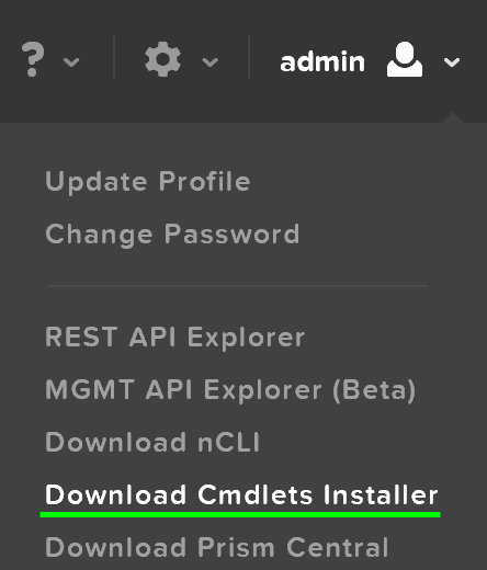
Download Nutanix CMDlets Installer The Nutanix CMDlets can be downloaded directly from the Prism UI (post 4.0.1) and can be found on the drop down in the upper right hand corner:
Load Nutanix Snappin
Check if snappin is loaded and if not, load
if ( (Get-PSSnapin -Name NutanixCmdletsPSSnapin -ErrorAction SilentlyContinue) -eq $null )
{
Add-PsSnapin NutanixCmdletsPSSnapin
}
List Nutanix CMDlets
Get-Command | Where-Object{$_.PSSnapin.Name -eq "NutanixCmdletsPSSnapin"}
Connect to a Acropolis Cluster
Connect-NutanixCluster -Server $server -UserName "myuser" -Password (Read-Host "Password: " -AsSecureString) -AcceptInvalidSSLCerts
Get Nutanix VMs matching a certain search string
Set to variable
$searchString = "myVM"
$vms = Get-NTNXVM | where {$_.vmName -match $searchString}
Interactive
Get-NTNXVM | where {$_.vmName -match "myString"}
Interactive and formatted
Get-NTNXVM | where {$_.vmName -match "myString"} | ft
Get Nutanix vDisks
Set to variable
$vdisks = Get-NTNXVDisk
Interactive
Get-NTNXVDisk
Interactive and formatted
Get-NTNXVDisk | ft
Get Nutanix Containers
Set to variable
$containers = Get-NTNXContainer
Interactive
Get-NTNXContainer
Interactive and formatted
Get-NTNXContainer | ft
Get Nutanix Protection Domains
Set to variable
$pds = Get-NTNXProtectionDomain
Interactive
Get-NTNXProtectionDomain
Interactive and formatted
Get-NTNXProtectionDomain | ft
Get Nutanix Consistency Groups
Set to variable
$cgs = Get-NTNXProtectionDomainConsistencyGroup
Interactive
Get-NTNXProtectionDomainConsistencyGroup
Interactive and formatted
Get-NTNXProtectionDomainConsistencyGroup | ft
Resources and Scripts:
- Nutanix Github - https://github.com/nutanix/Automation
- Manually Fingerprint vDisks - http://bit.ly/1syOqch
- vDisk Report - http://bit.ly/1r34MIT
- Protection Domain Report - http://bit.ly/1r34MIT
- Ordered PD Restore - http://bit.ly/1pyolrb
You can find more scripts on the Nutanix Github located at https://github.com/nutanix
Integrations
OpenStack
OpenStack is an open source platform for managing and building clouds. It is primarily broken into the front-end (dashboard and API) and infrastructure services (compute, storage, etc.).
The OpenStack and Nutanix solution is composed of a few main components:
- OpenStack Controller (OSC)
- An existing, or newly provisioned VM or host hosting the OpenStack UI, API and services. Handles all OpenStack API calls. In an Acropolis OVM deployment this can be co-located with the Acropolis OpenStack Drivers.
- Acropolis OpenStack Driver
- Responsible for taking OpenStack RPCs from the OpenStack Controller and translates them into native Acropolis API calls. This can be deployed on the OpenStack Controller, the OVM (pre-installed), or on a new VM.
- Acropolis OpenStack Services VM (OVM)
- VM with Acropolis drivers that is responsible for taking OpenStack RPCs from the OpenStack Controller and translates them into native Acropolis API calls.
The OpenStack Controller can be an existing VM / host, or deployed as part of the OpenStack on Nutanix solution. The Acropolis OVM is a helper VM which is deployed as part of the Nutanix OpenStack solution.
The client communicates with the OpenStack Controller using their expected methods (Web UI / HTTP, SDK, CLI or API) and the OpenStack controller communicates with the Acropolis OVM which translates the requests into native Acropolis REST API calls using the OpenStack Driver.
The figure shows a high-level overview of the communication:
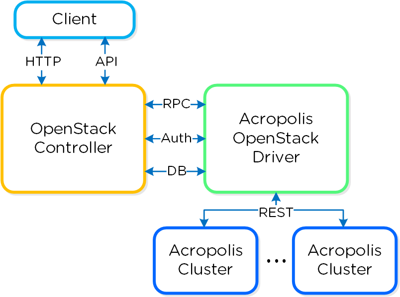
This allows for the best of both worlds, the goodness of the OpenStack Portal and APIs, without the complex OpenStack infrastructure and associated management. All back-end infrastructure services (compute, storage, network) leverage the native Nutanix services. No need to deploy Nova Compute hosts, etc. The platform exposes APIs for these services which the controller communicates with then translates them into native Acropolis API calls. Also, given the simplified deployment model, the full OpenStack + Nutanix solution can be up in less than 30 minutes.
Supported OpenStack Controllers
The current solution (as of 4.5.1) requires an OpenStack Controller on version Kilo or later.
The table shows a high-level conceptual role mapping:
| Item | Role | OpenStack Controller | Acropolis OVM | Acropolis Cluster | Prism |
|---|---|---|---|---|---|
| Tenant Dashboard | User interface and API | X | |||
| Admin Dashboard | Infra monitoring and ops | X | X | ||
| Orchestration | Object CRUD and lifecycle management | X | |||
| Quotas | Resource controls and limits | X | |||
| Users, Groups and Roles | Role based access control (RBAC) | X | |||
| SSO | Single-sign on | X | |||
| Platform Integration | OpenStack to Nutanix integration | X | |||
| Infrastructure Services | Target infrastructure (compute, storage, network) | X |
OpenStack Components
OpenStack is composed of a set of components which are responsible for serving various infrastructure functions. Some of these functions will be hosted by the OpenStack Controller and some will be hosted by the Acropolis OVM.
The table shows the core OpenStack components and role mapping:
| Component | Role | OpenStack Controller | Acropolis OVM |
|---|---|---|---|
| Keystone | Identity service | X | |
| Horizon | Dashboard and UI | X | |
| Nova | Compute | X | |
| Swift | Object storage | X | X |
| Cinder | Block storage | X | |
| Glance | Image service | X | X |
| Neutron | Networking | X | |
| Heat | Orchestration | X | |
| Others | All other components | X |
The figure shows a more detailed view of the OpenStack components and communication:
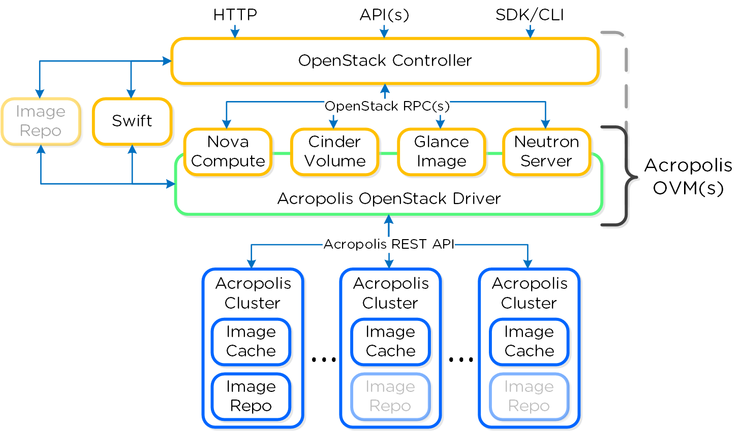
In the following sections we will go through some of the main OpenStack components and how they are integrated into the Nutanix platform.
Nova
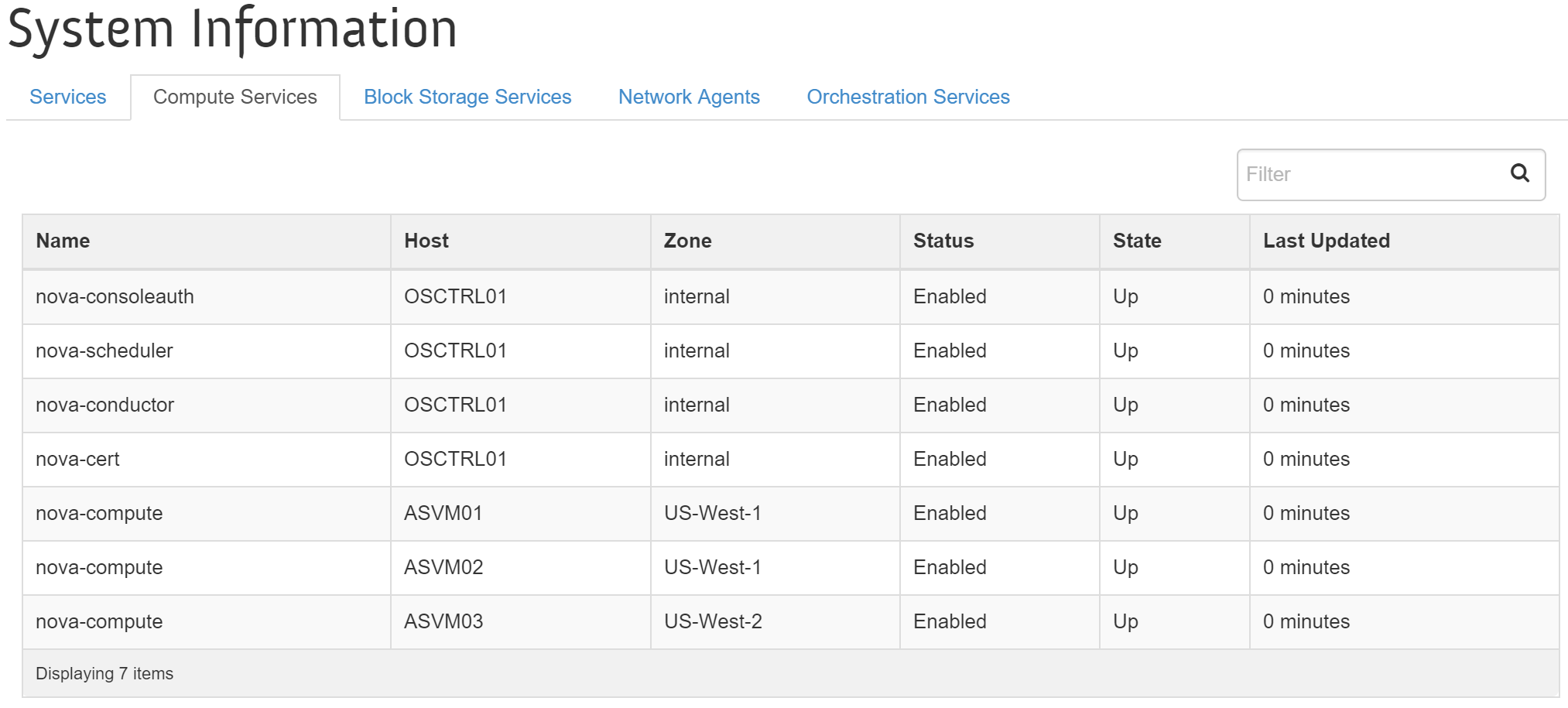
Nova is the compute engine and scheduler for the OpenStack platform. In the Nutanix OpenStack solution each Acropolis OVM acts as a compute host and every Acropolis Cluster will act as a single hypervisor host eligible for scheduling OpenStack instances. The Acropolis OVM runs the Nova-compute service.
You can view the Nova services using the OpenStack portal under 'Admin'->'System'->'System Information'->'Compute Services'.
The figure shows the Nova services, host and state:
The Nova scheduler decides which compute host (i.e. Acropolis OVM) to place the instances based upon the selected availability zone. These requests will be sent to the selected Acropolis OVM which will forward the request to the target host's (i.e. Acropolis cluster) Acropolis scheduler. The Acropolis scheduler will then determine optimal node placement within the cluster. Individual nodes within a cluster are not exposed to OpenStack.
You can view the compute and hypervisor hosts using the OpenStack portal under 'Admin'->'System'->'Hypervisors'.
The figure shows the Acropolis OVM as the compute host:
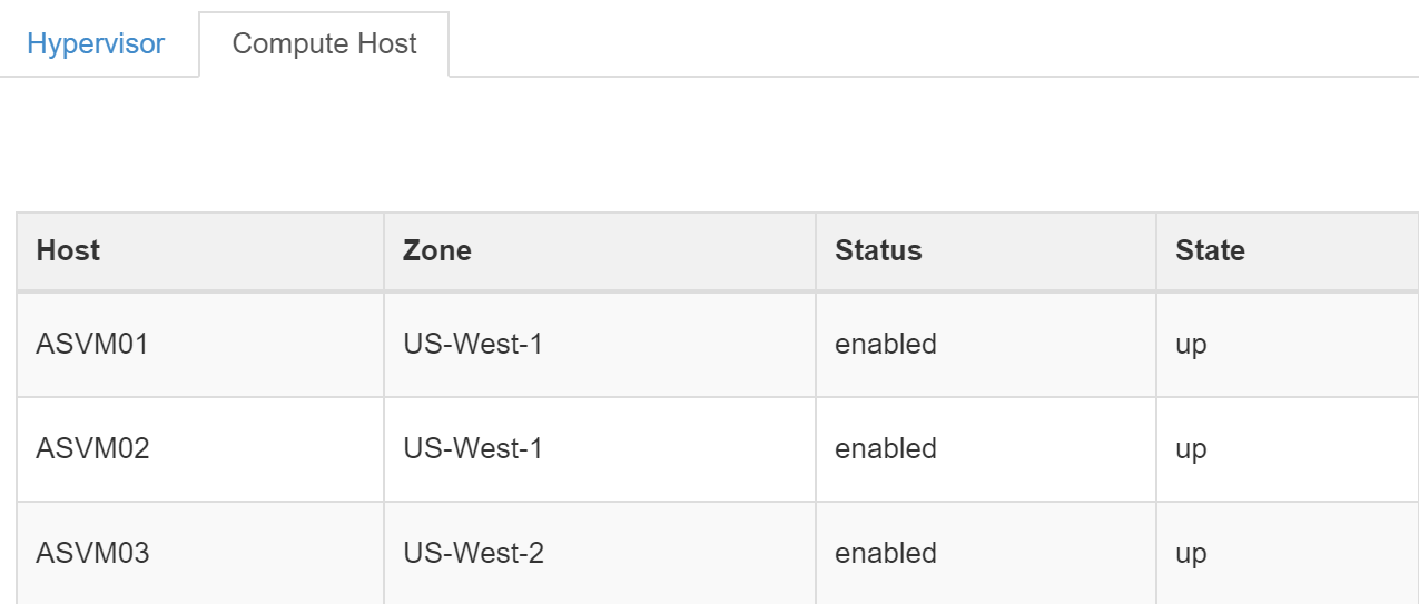
The figure shows the Acropolis cluster as the hypervisor host:
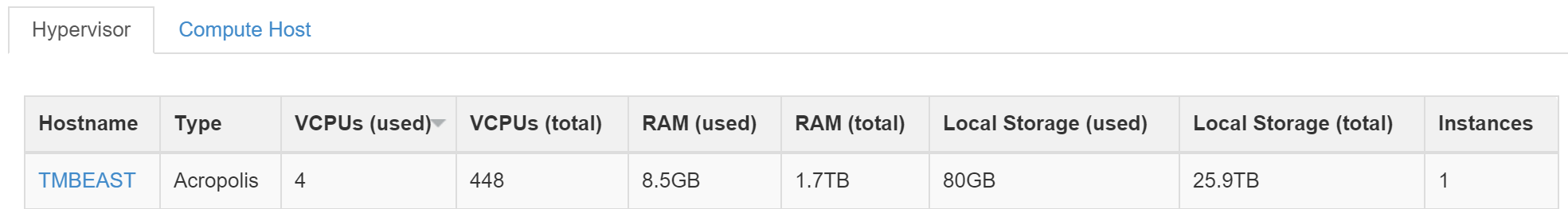
As you can see from the previous image the full cluster resources are seen in a single hypervisor host.
Swift
Swift in an object store used to store and retrieve files. This is currently only leveraged for backup / restore of snapshots and images.
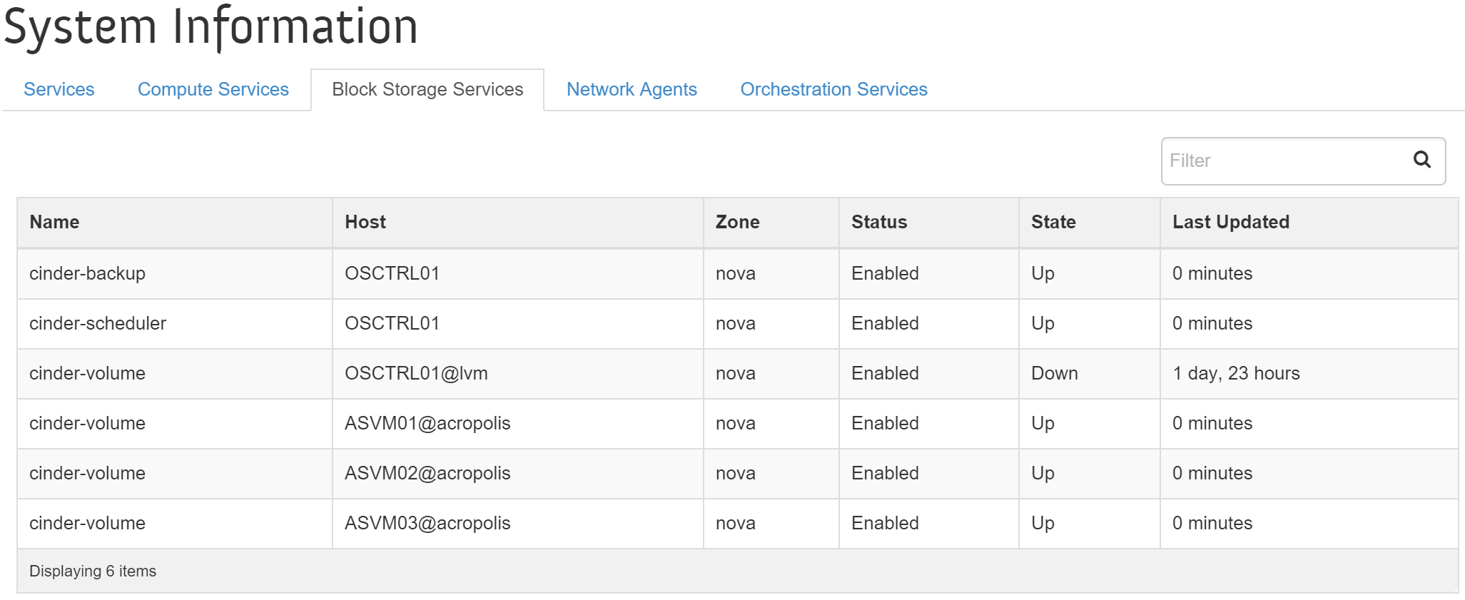
Cinder
Cinder is OpenStack's volume component for exposing iSCSI targets. Cinder leverages the Acropolis Volumes API in the Nutanix solution. These volumes are attached to the instance(s) directly as block devices (as compared to in-guest).
You can view the Cinder services using the OpenStack portal under 'Admin'->'System'->'System Information'->'Block Storage Services'.
The figure shows the Cinder services, host and state:
Glance / Image Repo
Glance is the image store for OpenStack and shows the available images for provisioning. Images can include ISOs, disks, and snapshots.
The Image Repo is the repository storing available images published by Glance. These can be located within the Nutanix environment or by an external source. When the images are hosted on the Nutanix platform, they will be published to the OpenStack controller via Glance on the OVM. In cases where the Image Repo exists only on an external source, Glance will be hosted by the OpenStack Controller and the Image Cache will be leveraged on the Acropolis Cluster(s).
Glance is enabled on a per-cluster basis and will always exist with the Image Repo. When Glance is enabled on multiple clusters the Image Repo will span those clusters and images created via the OpenStack Portal will be propagated to all clusters running Glance. Those clusters not hosting Glance will cache the images locally using the Image Cache.
Note
Pro tip
For larger deployments Glance should run on at least two Acropolis Clusters per site. This will provide Image Repo HA in the case of a cluster outage and ensure the images will always be available when not in the Image Cache.
When external sources host the Image Repo / Glance, Nova will be responsible for handling data movement from the external source to the target Acropolis Cluster(s). In this case the Image Cache will be leveraged on the target Acropolis Cluster(s) to cache the image locally for any subsequent provisioning requests for the image.
Neutron
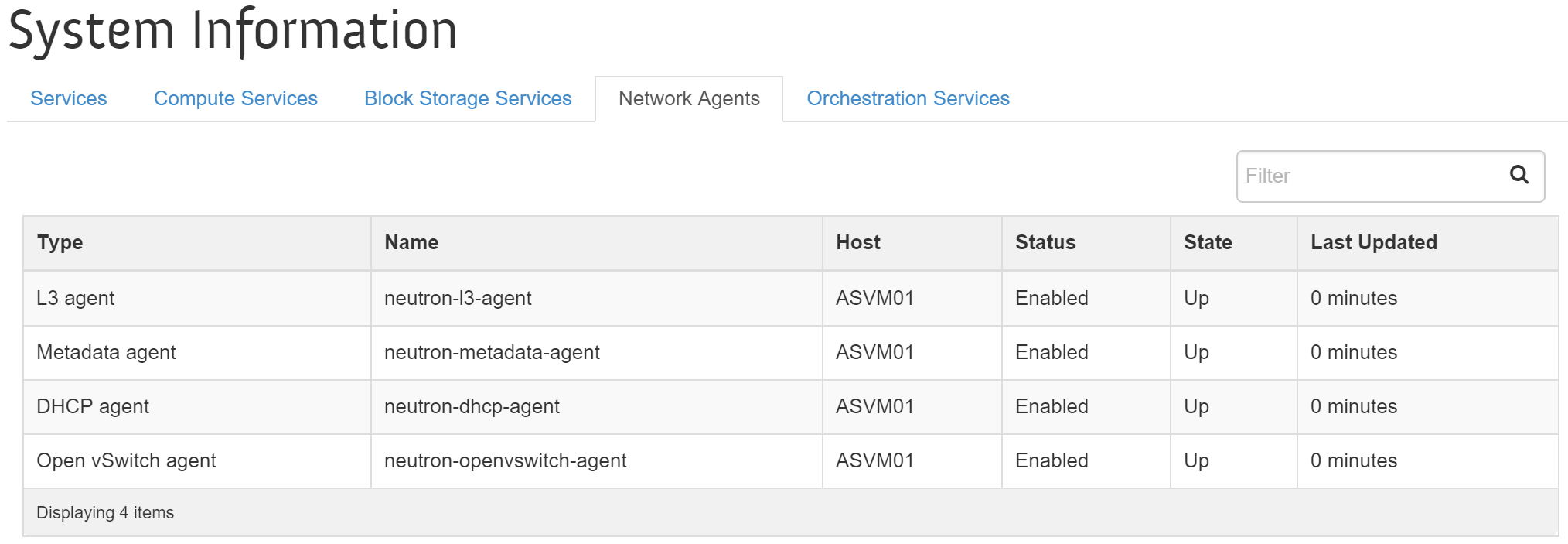
Neutron is the networking component of OpenStack and responsible for network configuration. The Acropolis OVM allows network CRUD operations to be performed by the OpenStack portal and will then make the required changes in Acropolis.
You can view the Neutron services using the OpenStack portal under 'Admin'->'System'->'System Information'->'Network Agents'.
The figure shows the Neutron services, host and state:
 + Currently only Local and VLAN network types are supported.
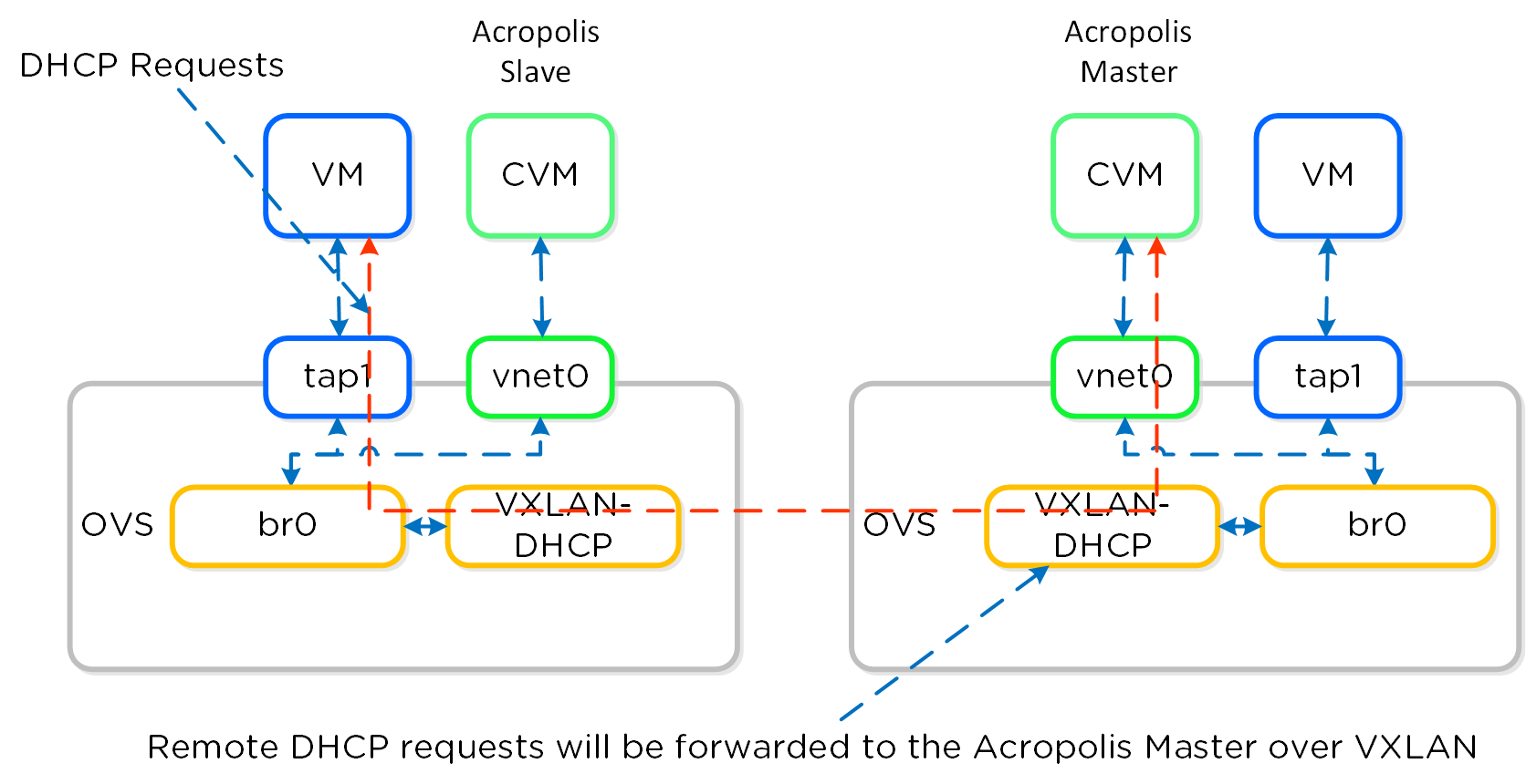
Neutron will assign IP addresses to instances when they are booted. In this case Acropolis will receive a desired IP address for the VM which will be allocated. When the VM performs a DHCP request the Acropolis Master will respond to the DHCP request on a private VXLAN as usual with AHV.
Note
Supported Network Types
Currently only Local and VLAN network types are supported.
The Keystone and Horizon components run in an OpenStack Controller which interfaces with the Acropolis OVM. The OVM(s) have an OpenStack Driver which is responsible for translating the OpenStack API calls into native Acropolis API calls.
Design and Deployment
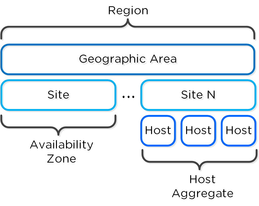
For large scale cloud deployments it is important to leverage a delivery topology that will be distributed and meet the requirements of the end-users while providing flexibility and locality.
OpenStack leverages the following high-level constructs which are defined below:
-
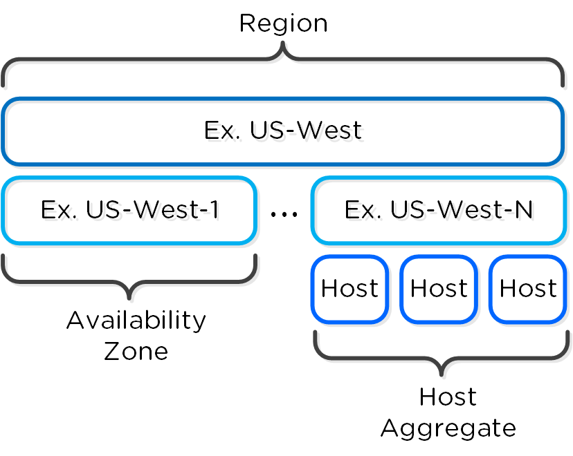
Region
- A geographic landmass or area where multiple Availability Zones (sites) are located. These can include regions like US-Northwest or US-West.
-
Availability Zone (AZ)
- A specific site or datacenter location where cloud services are hosted. These can include sites like US-Northwest-1 or US-West-1.
-
Host Aggregate
- A group of compute hosts, can be a row, aisle or equivalent to the site / AZ.
-
Compute Host
- An Acropolis OVM which is running the nova-compute service.
-
Hypervisor Host
- A Acropolis Cluster (seen as a single host).
The figure shows the high-level relationship of the constructs:
The figure shows an example application of the constructs:
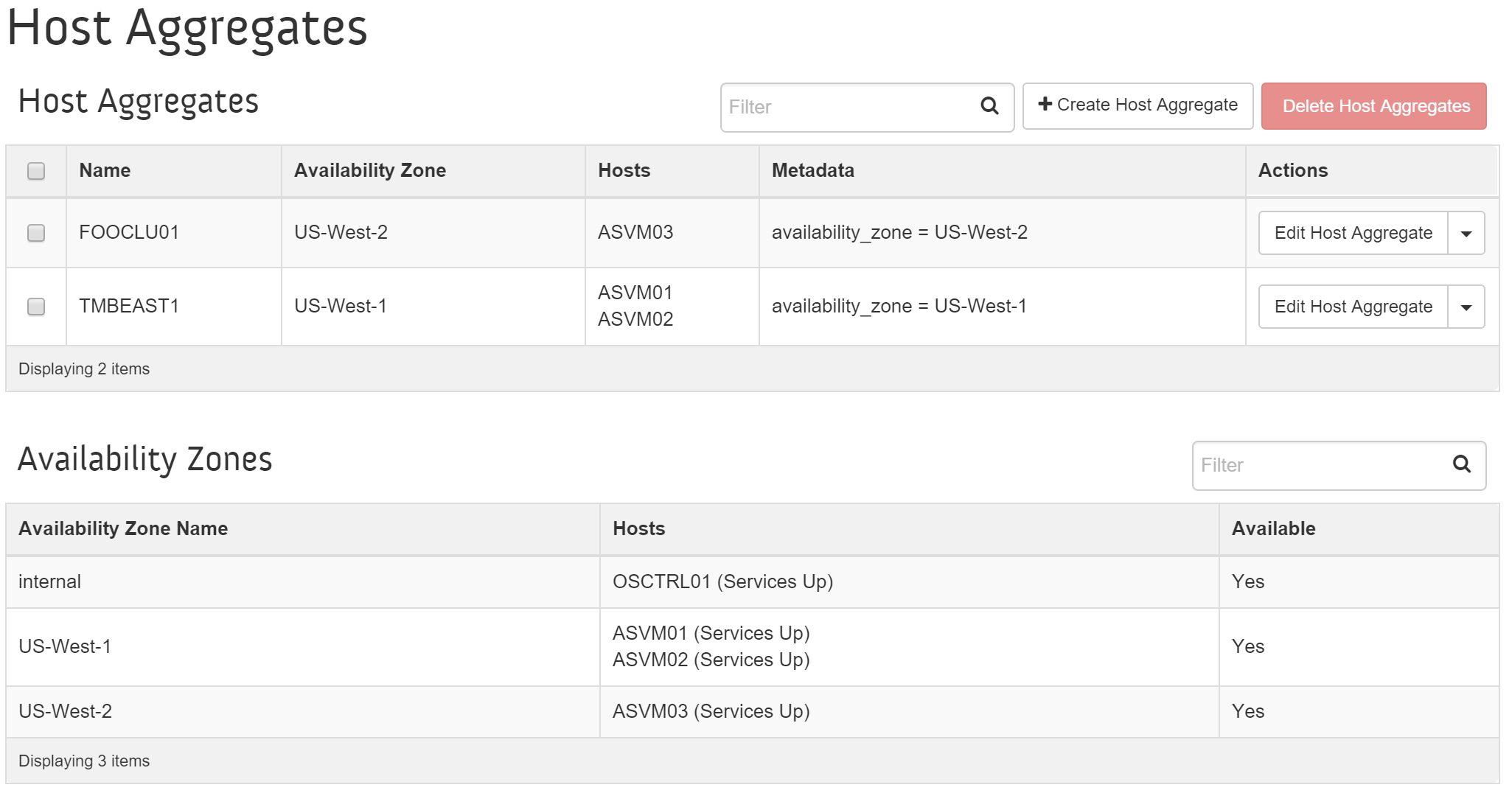
You can view and manage hosts, host aggregates and availability zones using the OpenStack portal under 'Admin'->'System'->'Host Aggregates'.
The figure shows the host aggregates, availability zones and hosts:
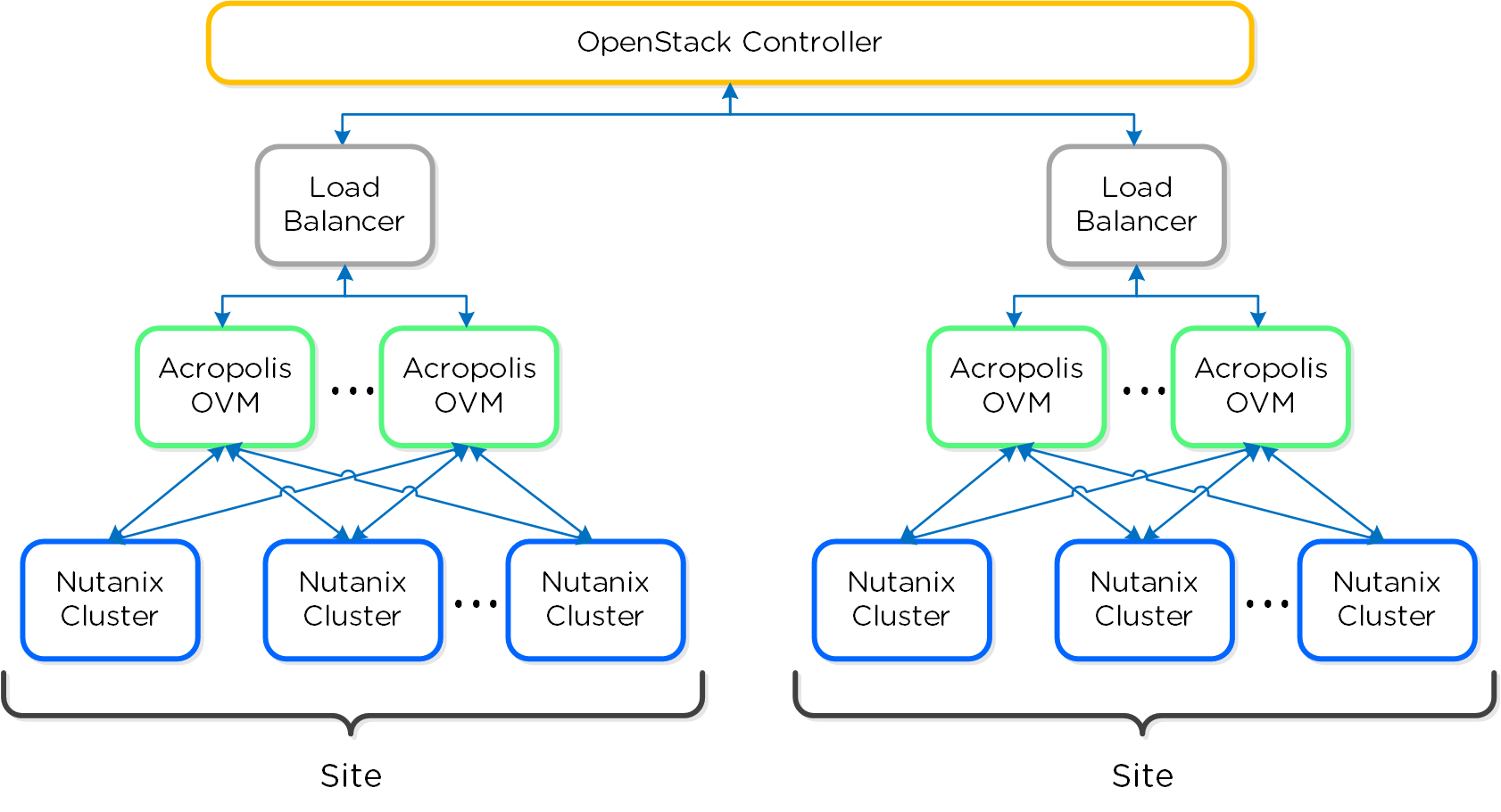
Services Design and Scaling
For larger deployments it is recommended to have multiple Acropolis OVMs connected to the OpenStack Controller abstracted by a load balancer. This allows for HA and of the OVMs as well as distribution of transactions. The OVM(s) don't contain any state information allowing them to be scaled.
The figure shows an example of scaling OVMs for a single site:
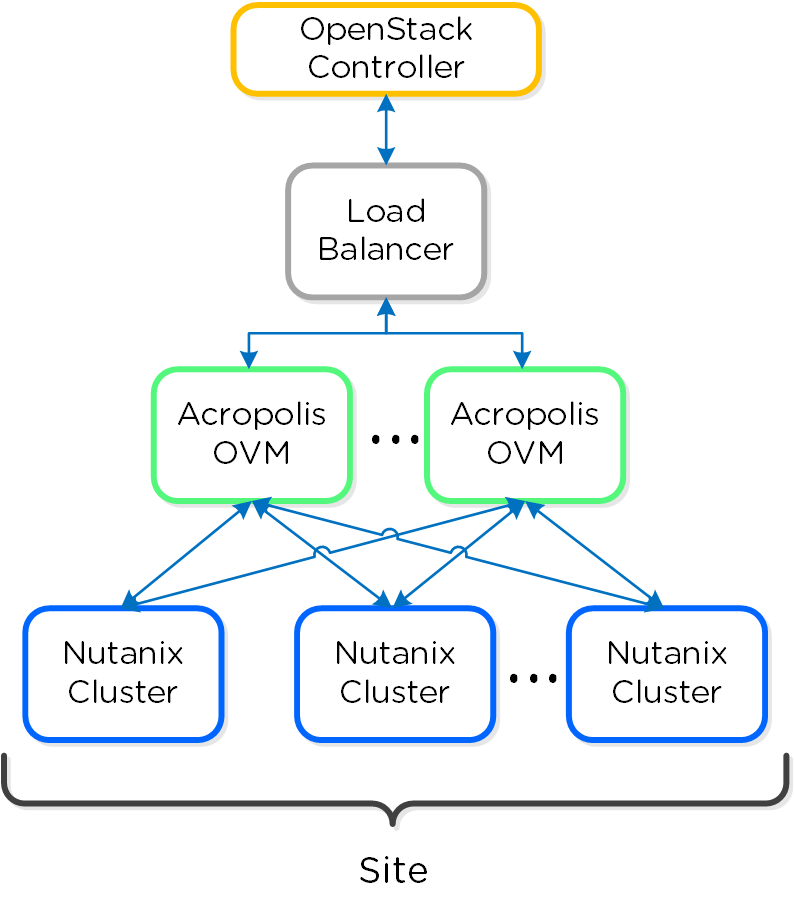
One method to achieve this for the OVM(s) is using Keepalived and HAproxy.
For environments spanning multiple sites the OpenStack Controller will talk to multiple Acropolis OVMs across sites.
The figure shows an example of the deployment across multiple sites:
Deployment
The OVM can be deployed as a standalone RPM on a CentOS / Redhat distro or as a full VM. The Acropolis OVM can be deployed on any platform (Nutanix or non-Nutanix) as long as it has network connectivity to the OpenStack Controller and Nutanix Cluster(s).
The VM(s) for the Acropolis OVM can be deployed on a Nutanix AHV cluster using the following steps. If the OVM is already deployed you can skip past the VM creation steps. You can use the full OVM image or use an existing CentOS / Redhat VM image.
First we will import the provided Acropolis OVM disk image to Acropolis cluster. This can be done by copying the disk image over using SCP or by specifying a URL to copy the file from. We will cover importing this using the Images API. Note: It is possible to deploy this VM anywhere, not necessarily on a Acropolis cluster.
To import the disk image using Images API, run the following command:
image.create <IMAGE_NAME> source_url=<SOURCE_URL> container=<CONTAINER_NAME>
Next create the Acropolis VM for the OVM by running the following ACLI commands on any CVM:
vm.create <VM_NAME> num_vcpus=2 memory=16G
vm.disk_create <VM_NAME> clone_from_image=<IMAGE_NAME>
vm.nic_create <VM_NAME> network=<NETWORK_NAME>
vm.on <VM_NAME>
Once the VM(s) have been created and powered on, SSH to the OVM(s) using the provided credentials.
Note
OVMCTL Help
Help txt can be displayed by running the following command on the OVM:
ovmctl --help
The OVM supports two deployment modes:
-
OVM-allinone
- OVM includes all Acropolis drivers and OpenStack controller
-
OVM-services
- OVM includes all Acropolis drivers and communicates with external/remote OpenStack controller
Both deployment modes will be covered in the following sections. You can use in any mode and also switch between modes.
OVM-allinone
The following steps cover the OVM-allinone deployment. Start by SSHing to the OVM(s) to run the following commands.
# Register OpenStack Driver service
ovmctl --add ovm --name <OVM_NAME> --ip <OVM_IP> --netmask <NET_MASK> --gateway <DEFAULT_GW> --domain <DOMAIN> --nameserver <DNS>
# Register OpenStack Controller
ovmctl --add controller --name <OVM_NAME> --ip <OVM_IP>
# Register Acropolis Cluster(s) (run for each cluster to add)
ovmctl --add cluster --name <CLUSTER_NAME> --ip <CLUSTER_IP> --username <PRISM_USER> --password <PRISM_PASSWORD>
The following values are used as defaults:
Number of VCPUs per core = 4
Container name = default
Image cache = disabled, Image cache URL = None
Next we'll verify the configuration using the following command:
ovmctl --show
At this point everything should be up and running, enjoy.
OVM-services
The following steps cover the OVM-services deployment. Start by SSHing to the OVM(s) to run the following commands.
# Register OpenStack Driver service
ovmctl --add ovm --name <OVM_NAME> --ip <OVM_IP>
# Register OpenStack Controller
ovmctl --add controller --name <OS_CONTROLLER_NAME> --ip <OS_CONTROLLER_IP> --username <OS_CONTROLLER_USERNAME> --password <OS_CONTROLLER_PASSWORD>
The following values are used as defaults:
Authentication: auth_strategy = keystone, auth_region = RegionOne
auth_tenant = services, auth_password = admin
Database: db_{nova,cinder,glance,neutron} = mysql, db_{nova,cinder,glance,neutron}_password = admin
RPC: rpc_backend = rabbit, rpc_username = guest, rpc_password = guest
# Register Acropolis Cluster(s) (run for each cluster to add)
ovmctl --add cluster --name <CLUSTER_NAME> --ip <CLUSTER_IP> --username <PRISM_USER> --password <PRISM_PASSWORD>
The following values are used as defaults:
Number of VCPUs per core = 4
Container name = default
Image cache = disabled, Image cache URL = None
If non-default passwords were used for the OpenStack controller deployment, we'll need to update those:
# Update controller passwords (if non-default are used)
ovmctl --update controller --name <OS_CONTROLLER_NAME> --auth_nova_password <> --auth_glance_password <> --auth_neutron_password <> --auth_cinder_password <> --db_nova_password <> --db_glance_password <> --db_neutron_password <> --db_cinder_password <>
Next we'll verify the configuration using the following command:
ovmctl --show
Now that the OVM has been configured, we'll configure the OpenStack Controller to know about the Glance and Neutron endpoints.
Log in to the OpenStack controller and enter the keystonerc_admin source:
# enter keystonerc_admin
source ./keystonerc_admin
First we will delete the existing endpoint for Glance that is pointing to the controller:
# Find old Glance endpoint id (port 9292)
keystone endpoint-list
# Remove old keystone endpoint for Glance
keystone endpoint-delete <GLANCE_ENDPOINT_ID>
Next we will create the new Glance endpoint that will point to the OVM:
# Find Glance service id
keystone service-list | grep glance
# Will look similar to the following:
| 9e539e8dee264dd9a086677427434982 | glance | image |
# Add Keystone endpoint for Glance
keystone endpoint-create \
--service-id <GLANCE_SERVICE_ID> \
--publicurl http://<OVM_IP>:9292 \
--internalurl http://<OVM_IP>:9292 \
--region <REGION_NAME> \
--adminurl http://<OVM_IP>:9292
Next we will delete the existing endpoint for Neutron that is pointing to the controller:
# Find old Neutron endpoint id (port 9696)
keystone endpoint-list
# Remove old keystone endpoint for Neutron
keystone endpoint-delete <NEUTRON_ENDPOINT_ID>
Next we will create the new Neutron endpoint that will point to the OVM:
# Find Neutron service id
keystone service-list | grep neutron
# Will look similar to the following:
| f4c4266142c742a78b330f8bafe5e49e | neutron | network |
# Add Keystone endpoint for Neutron
keystone endpoint-create \
--service-id <NEUTRON_SERVICE_ID> \
--publicurl http://<OVM_IP>:9696 \
--internalurl http://<OVM_IP>:9696 \
--region <REGION_NAME> \
--adminurl http://<OVM_IP>:9696
After the endpoints have been created we will update the Nova and Cinder configuration files with new Acropolis OVM IP of Glance host.
First we will edit Nova.conf which is located at /etc/nova/nova.conf and edit the following lines:
[glance]
...
# Default glance hostname or IP address (string value)
host=<OVM_IP>
# Default glance port (integer value)
port=9292
...
# A list of the glance api servers available to nova. Prefix
# with https:// for ssl-based glance api servers.
# ([hostname|ip]:port) (list value)
api_servers=<OVM_IP>:9292
Now we will disable nova-compute on the OpenStack controller (if not already):
systemctl disable openstack-nova-compute.service
systemctl stop openstack-nova-compute.service
service openstack-nova-compute stop
Next we will edit Cinder.conf which is located at /etc/cinder/cinder.conf and edit the following items:
# Default glance host name or IP (string value)
glance_host=<OVM_IP>
# Default glance port (integer value)
glance_port=9292
# A list of the glance API servers available to cinder
# ([hostname|ip]:port) (list value)
glance_api_servers=$glance_host:$glance_port
We will also comment out lvm enabled backends as those will not be leveraged:
# Comment out the following lines in cinder.conf
#enabled_backends=lvm
#[lvm]
#iscsi_helper=lioadm
#volume_group=cinder-volumes
#iscsi_ip_address=
#volume_driver=cinder.volume.drivers.lvm.LVMVolumeDriver
#volumes_dir=/var/lib/cinder/volumes
#iscsi_protocol=iscsi
#volume_backend_name=lvm
Now we will disable cinder volume on the OpenStack controller (if not already):
systemctl disable openstack-cinder-volume.service
systemctl stop openstack-cinder-volume.service
service openstack-cinder-volume stop
Now we will disable glance-image on the OpenStack controller (if not already):
systemctl disable openstack-glance-api.service
systemctl disable openstack-glance-registry.service
systemctl stop openstack-glance-api.service
systemctl stop openstack-glance-registry.service
service openstack-glance-api stop
service openstack-glance-registry stop
After the files have been edited we will restart the Nova and Cinder services to take the new configuration settings. The services can be restarted with the following commands below or by running the scripts which are available for download.
# Restart Nova services
service openstack-nova-api restart
service openstack-nova-consoleauth restart
service openstack-nova-scheduler restart
service openstack-nova-conductor restart
service openstack-nova-cert restart
service openstack-nova-novncproxy restart
# OR you can also use the script which can be downloaded as part of the helper tools:
~/openstack/commands/nova-restart
# Restart Cinder
service openstack-cinder-api restart
service openstack-cinder-scheduler restart
service openstack-cinder-backup restart
# OR you can also use the script which can be downloaded as part of the helper tools:
~/openstack/commands/cinder-restart
Troubleshooting & Advanced Administration
Key log locations
| Component | Key Log Location(s) |
|---|---|
| Keystone | /var/log/keystone/keystone.log |
| Horizon | /var/log/horizon/horizon.log |
| Nova | /var/log/nova/nova-api.log /var/log/nova/nova-scheduler.log /var/log/nova/nove-compute.log* |
| Swift | /var/log/swift/swift.log |
| Cinder | /var/log/cinder/api.log /var/log/cinder/scheduler.log /var/log/cinder/volume.log |
| Glance | /var/log/glance/api.log /var/log/glance/registry.log |
| Neutron | /var/log/neutron/server.log /var/log/neutron/dhcp-agent.log* /var/log/neutron/l3-agent.log* /var/log/neutron/metadata-agent.log* /var/log/neutron/openvswitch-agent.log* |
Logs marked with * are on the Acropolis OVM only.
Note
Pro tip
Check NTP if a service is seen as state 'down' in OpenStack Manager (Admin UI or CLI) even though the service is running in the OVM. Many services have a requirement for time to be in sync between the OpenStack Controller and Acropolis OVM.
Command Reference
Load Keystone source (perform before running other commands)
source keystonerc_admin
List Keystone services
keystone service-list
List Keystone endpoints
keystone endpoint-list
Create Keystone endpoint
keystone endpoint-create \
--service-id=<SERVICE_ID> \
--publicurl=http://<IP:PORT> \
--internalurl=http://<IP:PORT> \
--region=<REGION_NAME> \
--adminurl=http://<IP:PORT>
List Nova instances
nova list
Show instance details
nova show <INSTANCE_NAME>
List Nova hypervisor hosts
nova hypervisor-list
Show hypervisor host details
nova hypervisor-show <HOST_ID>
List Glance images
glance image-list
Show Glance image details
glance image-show <IMAGE_ID>
Part III. Book of Acropolis
a·crop·o·lis - /ɘ ' kräpɘlis/ - noun - data plane
storage, compute and virtualization platform.
Architecture
Acropolis is a distributed multi-resource manager, orchestration platform and data plane.
It is broken down into three main components:
- Distributed Storage Fabric (DSF)
- This is at the core and birth of the Nutanix platform and expands upon the Nutanix Distributed Filesystem (NDFS). NDFS has now evolved from a distributed system pooling storage resources into a much larger and capable storage platform.
- App Mobility Fabric (AMF)
- Hypervisors abstracted the OS from hardware, and the AMF abstracts workloads (VMs, Storage, Containers, etc.) from the hypervisor. This will provide the ability to dynamically move the workloads between hypervisors, clouds, as well as provide the ability for Nutanix nodes to change hypervisors.
- Hypervisor
- A multi-purpose hypervisor based upon the CentOS KVM hypervisor.
Building upon the distributed nature of everything Nutanix does, we’re expanding this into the virtualization and resource management space. Acropolis is a back-end service that allows for workload and resource management, provisioning, and operations. Its goal is to abstract the facilitating resource (e.g., hypervisor, on-premise, cloud, etc.) from the workloads running, while providing a single “platform” to operate.
This gives workloads the ability to seamlessly move between hypervisors, cloud providers, and platforms.
The figure highlights an image illustrating the conceptual nature of Acropolis at various layers:
Note
Supported Hypervisors for VM Management
As of 4.7, AHV and ESXi are the supported hypervisors for VM management, however this may expand in the future. The Volumes API and read-only operations are still supported on all.
Hyperconverged Platform
For a video explanation you can watch the following video: LINK
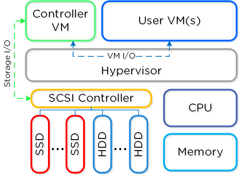
The Nutanix solution is a converged storage + compute solution which leverages local components and creates a distributed platform for virtualization, also known as a virtual computing platform. The solution is a bundled hardware + software appliance which houses 2 (6000/7000 series) or 4 nodes (1000/2000/3000/3050 series) in a 2U footprint.
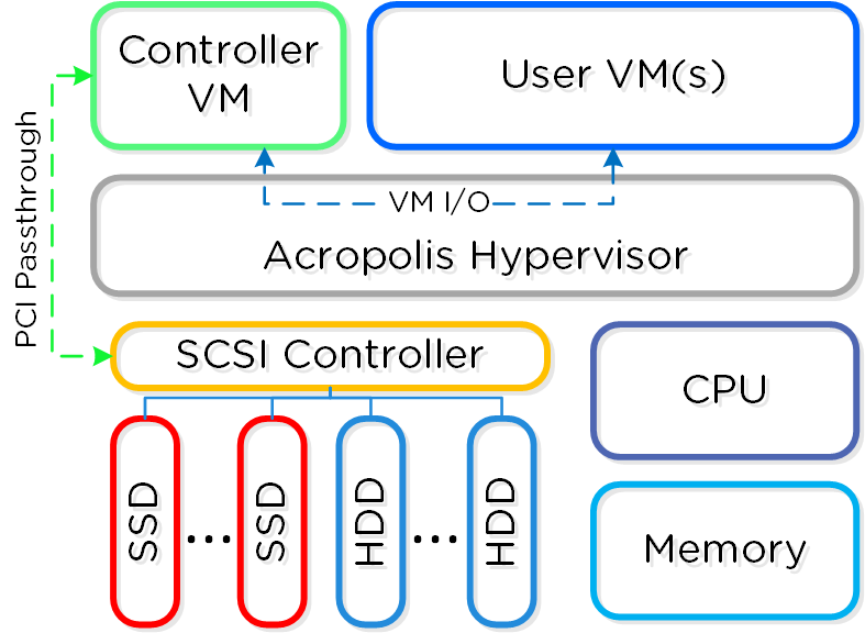
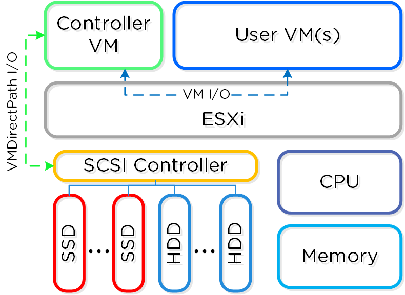
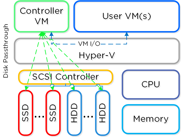
Each node runs an industry-standard hypervisor (ESXi, KVM, Hyper-V currently) and the Nutanix Controller VM (CVM). The Nutanix CVM is what runs the Nutanix software and serves all of the I/O operations for the hypervisor and all VMs running on that host. For the Nutanix units running VMware vSphere, the SCSI controller, which manages the SSD and HDD devices, is directly passed to the CVM leveraging VM-Direct Path (Intel VT-d). In the case of Hyper-V, the storage devices are passed through to the CVM.
The following figure provides an example of what a typical node logically looks like:
Distributed System
Together, a group of Nutanix nodes forms a distributed system (Nutanix cluster) responsible for providing the Prism and Acropolis capabilities. All services and components are distributed across all CVMs in a cluster to provide for high-availability and linear performance at scale.
The following figure shows an example of how these Nutanix nodes form a Nutnaix cluster:
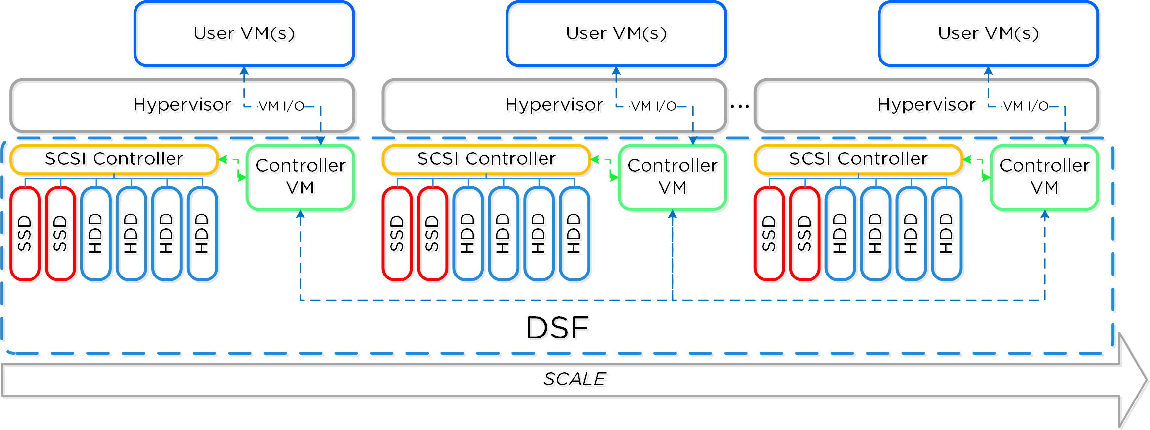
Software-Defined
As mentioned above (likely numerous times), the Nutanix platform is a software-based solution which ships as a bundled software + hardware appliance. The controller VM is where the vast majority of the Nutanix software and logic sits and was designed from the beginning to be an extensible and pluggable architecture. A key benefit to being software-defined and not relying upon any hardware offloads or constructs is around extensibility. As with any product life cycle, advancements and new features will always be introduced.
By not relying on any custom ASIC/FPGA or hardware capabilities, Nutanix can develop and deploy these new features through a simple software update. This means that the deployment of a new feature (e.g., deduplication) can be deployed by upgrading the current version of the Nutanix software. This also allows newer generation features to be deployed on legacy hardware models. For example, say you’re running a workload running an older version of Nutanix software on a prior generation hardware platform (e.g., 2400). The running software version doesn’t provide deduplication capabilities which your workload could benefit greatly from. To get these features, you perform a rolling upgrade of the Nutanix software version while the workload is running, and you now have deduplication. It’s really that easy.
Similar to features, the ability to create new “adapters” or interfaces into DSF is another key capability. When the product first shipped, it solely supported iSCSI for I/O from the hypervisor, this has now grown to include NFS and SMB. In the future, there is the ability to create new adapters for various workloads and hypervisors (HDFS, etc.). And again, all of this can be deployed via a software update. This is contrary to most legacy infrastructures, where a hardware upgrade or software purchase is normally required to get the “latest and greatest” features. With Nutanix, it’s different. Since all features are deployed in software, they can run on any hardware platform, any hypervisor, and be deployed through simple software upgrades.
The following figure shows a logical representation of what this software-defined controller framework looks like:
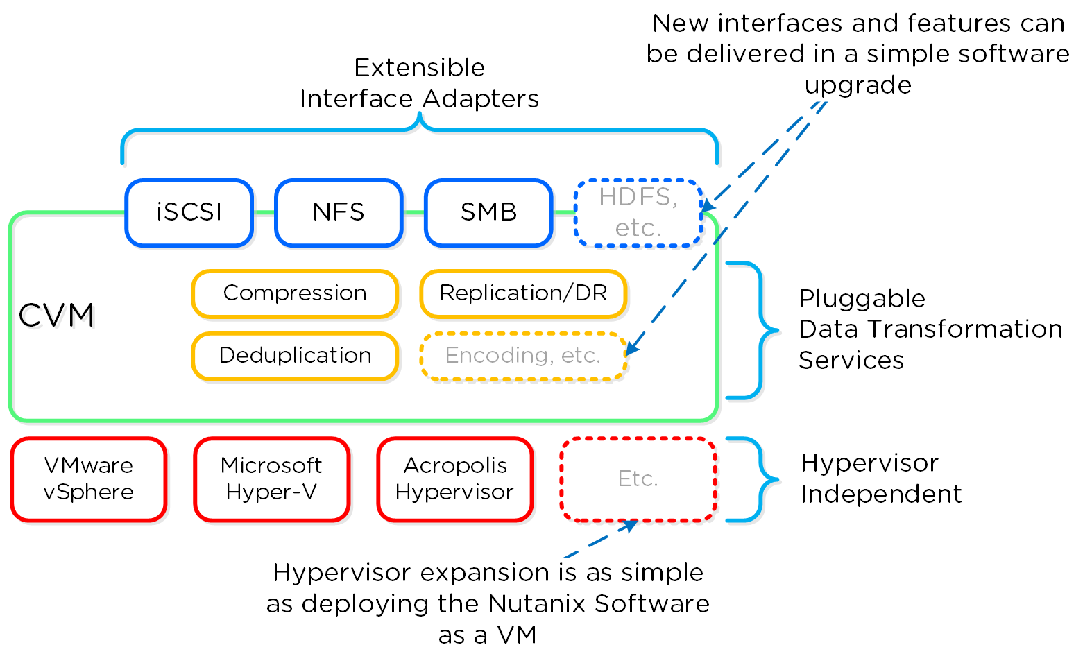
Cluster Components
For a visual explanation you can watch the following video: LINK
The user-facing Nutanix product is extremely simple to deploy and use. This is primarily possible through abstraction and a lot of automation / integration in the software.
The following is a detailed view of the main Nutanix Cluster components (don't worry, no need to memorize or know what everything does):
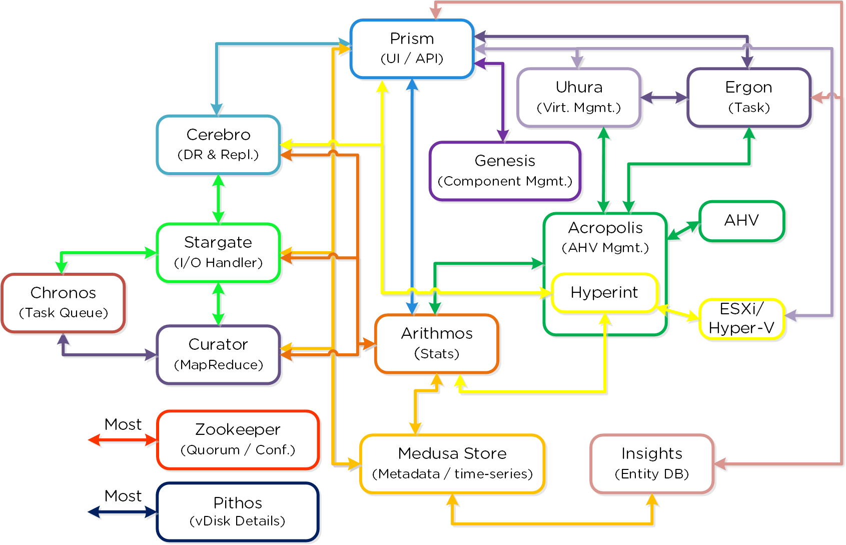
Cassandra
- Key Role: Distributed metadata store
- Description: Cassandra stores and manages all of the cluster metadata in a distributed ring-like manner based upon a heavily modified Apache Cassandra. The Paxos algorithm is utilized to enforce strict consistency. This service runs on every node in the cluster. The Cassandra is accessed via an interface called Medusa.
Zookeeper
- Key Role: Cluster configuration manager
- Description: Zookeeper stores all of the cluster configuration including hosts, IPs, state, etc. and is based upon Apache Zookeeper. This service runs on three nodes in the cluster, one of which is elected as a leader. The leader receives all requests and forwards them to its peers. If the leader fails to respond, a new leader is automatically elected. Zookeeper is accessed via an interface called Zeus.
Stargate
- Key Role: Data I/O manager
- Description: Stargate is responsible for all data management and I/O operations and is the main interface from the hypervisor (via NFS, iSCSI, or SMB). This service runs on every node in the cluster in order to serve localized I/O.
Curator
- Key Role: MapReduce cluster management and cleanup
- Description: Curator is responsible for managing and distributing tasks throughout the cluster, including disk balancing, proactive scrubbing, and many more items. Curator runs on every node and is controlled by an elected Curator Master who is responsible for the task and job delegation. There are two scan types for Curator, a full scan which occurs around every 6 hours and a partial scan which occurs every hour.
Prism
- Key Role: UI and API
- Description: Prism is the management gateway for component and administrators to configure and monitor the Nutanix cluster. This includes Ncli, the HTML5 UI, and REST API. Prism runs on every node in the cluster and uses an elected leader like all components in the cluster.
Genesis
- Key Role: Cluster component & service manager
- Description: Genesis is a process which runs on each node and is responsible for any services interactions (start/stop/etc.) as well as for the initial configuration. Genesis is a process which runs independently of the cluster and does not require the cluster to be configured/running. The only requirement for Genesis to be running is that Zookeeper is up and running. The cluster_init and cluster_status pages are displayed by the Genesis process.
Chronos
- Key Role: Job and task scheduler
- Description: Chronos is responsible for taking the jobs and tasks resulting from a Curator scan and scheduling/throttling tasks among nodes. Chronos runs on every node and is controlled by an elected Chronos Master that is responsible for the task and job delegation and runs on the same node as the Curator Master.
Cerebro
- Key Role: Replication/DR manager
- Description: Cerebro is responsible for the replication and DR capabilities of DSF. This includes the scheduling of snapshots, the replication to remote sites, and the site migration/failover. Cerebro runs on every node in the Nutanix cluster and all nodes participate in replication to remote clusters/sites.
Pithos
- Key Role: vDisk configuration manager
- Description: Pithos is responsible for vDisk (DSF file) configuration data. Pithos runs on every node and is built on top of Cassandra.
Acropolis Services
An Acropolis Slave runs on every CVM with an elected Acropolis Master which is responsible for task scheduling, execution, IPAM, etc. Similar to other components which have a Master, if the Acropolis Master fails, a new one will be elected.
The role breakdown for each can be seen below:
- Acropolis Master
- Task scheduling & execution
- Stat collection / publishing
- Network Controller (for hypervisor)
- VNC proxy (for hypervisor)
- HA (for hypervisor)
- Acropolis Slave
- Stat collection / publishing
- VNC proxy (for hypervisor)
Here we show a conceptual view of the Acropolis Master / Slave relationship:
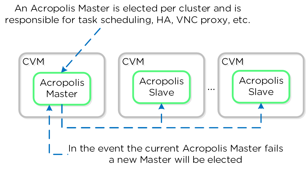
Dynamic Scheduler
Efficient scheduling of resources is critical to ensure resources are effectively consumed. The Acropolis Dynamic Scheduler extends the traditional means of scheduling that relies upon compute utilization (CPU/MEM) to make placement decisions. It leverages compute, as well as storage and others to drive VM and volume (ABS) placement decisions. This ensures that resources are effectively consumed and end-user performance is optimal.
Resource scheduling can be broken down into two key areas:
-
Initial placement
- Where an item is scheduled at power-on
-
Runtime Optimization
- Movement of workloads based upon runtime metrics
The original Acropolis Scheduler had taken care of the initial placement decisions since its release. With its release in Asterix, the Acropolis Dynamic Scheduler expands upon this to provide runtime resources optimization.
The figure shows a high-level view of the scheduler architecture:
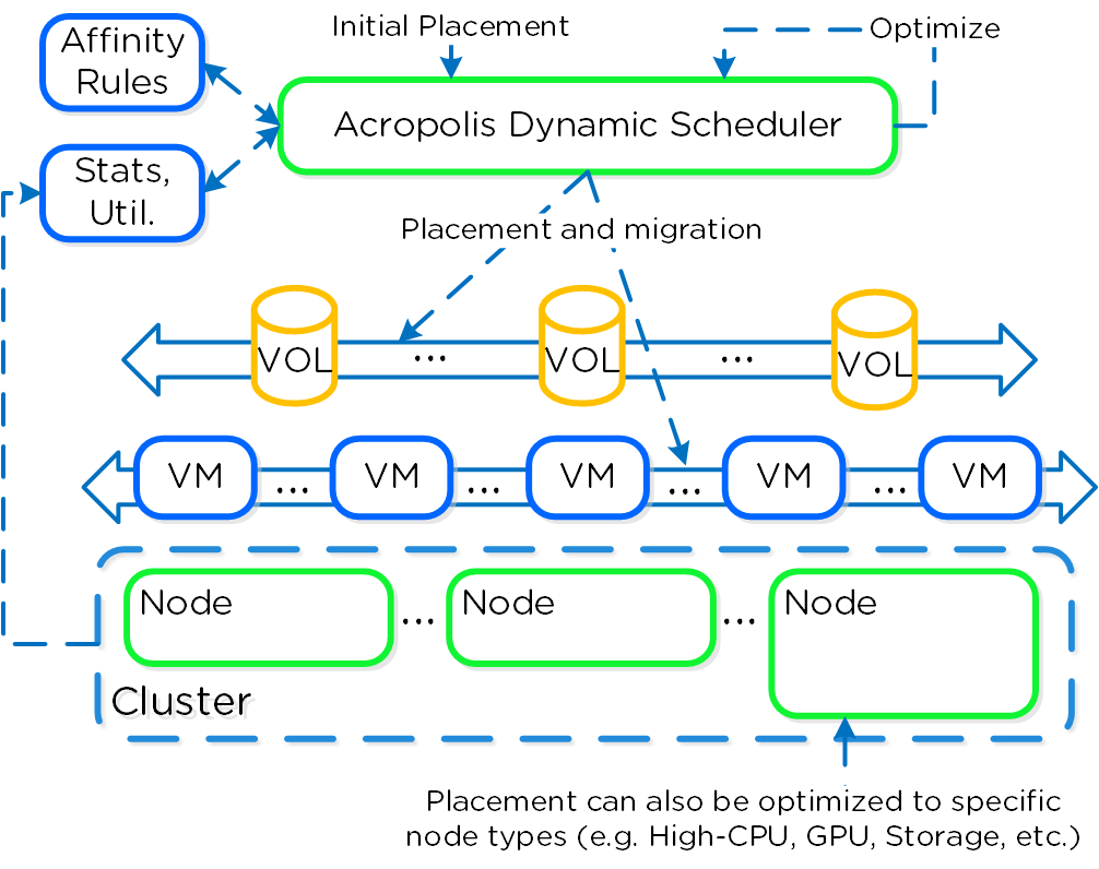
The dynamic scheduler runs consistently throughout the day to optimize placement (currently every 15 minutes | lazan_anomaly_detection_period_secs). Estimated demand is calculated using historical utilization values and fed into a smoothing algorithm. This estimated demand is what is used to determine movement, which insures a sudden spike will not skew decisions.
Note
A different approach towards resource optimization
When you look at existing scheduling / optimization platforms (VMware DRS, Microsoft PRO) they are all focused on balancing workloads evenly across cluster resources.
For example, say we had 3 hosts in a cluster, each of which is utilized 50%, 5%, 5% respectively. Typical solutions would try to re-balance workloads to get each hosts utilization ~20%. But why?
What we're really trying to do is eliminate / negate any contention for resources, not eliminate skew. Unless there is contention for resources there is no positive gain from "balancing" workloads. In fact by forcing unecessary movement we cause additional requisite work (e.g. memory transfer, cache re-localization, etc.), all of which consumes resources.
The Acroplis Dynamic Scheduler does just this, it will only invoke workload movement if there is expected contention for resources, not because of skew. NOTE: Acropolis DSF works in a different way and works to ensure uniform distribution of data throughout the cluster to eliminate hot spots and speed up rebuilds. To learn more of DSF, check out the 'disk balancing' section.
Placement Decisions
Placement decisions are based upon the following items:
-
Compute utilization
- We monitor each individual node's compute utilization. In the event where a node's expected CPU allocation breaches its threshold (currently 85% of host CPU | lazan_host_cpu_usage_threshold_fraction) we will migrate VMs off those host(s) to re-balance the workload. A key thing to mention here is a migration will only be performed when there is contention. If there is skew in utilization between nodes (e.g. 3 nodes at 10% and 1 at 50%) we will not perform a migration as there is no benefit from doing so until there is contention for resources.
-
Storage performance
- Being a hyperconverged platform we manage both compute and storage resources. The scheduler will monitor each node's Stargate process utilization. In the event where certain Stargate(s) breach their allocation threshold (currently 85% of CPU allocated to Stargate | lazan_stargate_cpu_usage_threshold_pct) , we will migrate resources across hosts to eliminate any hot spots. Both VMs and ABS Volumes can be migrated to eliminate any hot Stargates.
-
[Anti-]Affinity rules
- Affinity or Anti-affinity constraints determine where certain resources are scheduled based upon other resources in the environment. In certain cases you want VMs to run on the same node for licensing reasons. In this case the VMs would be affined to the same host. In other cases you might want to ensure VMs run on different nodes for availability purposes. In this case the VMs would be anti-affined.
The scheduler will make its best effort to optimize workload placement based upon the prior items. The system places a penalty on movement to ensure not too many migrations are taking place. This is a key item as we want to make sure the movement doesn't have any negative impacts on the workload.
After a migration the system will judge it's "effectiveness" and see what the actual benefit is. This learning model can self-optimize to ensure there is a valid basis for any migration decision.
Security and Encryption
Security
Security is a core part of the Nutanix platform and was kept in mind from day one. The Nutanix Security Development Lifecycle (SecDL) incorporates security into every step of the development process. The system ships secure from the factory, rather than being an afterthought requiring end-users to "harden" the platform.
The Nutanix platform has the following security certifications / qualifications:
-
Common Criteria
- Common Criteria was produced predominantly so that companies selling computer products for the government market (mainly for Defense or Intelligence use) would only need to have them evaluated against one set of standards. The CC was developed by the governments of Canada, France, Germany, the Netherlands, the UK, and the U.S.
-
Security Technical Implementation Guides (STIGs)
- Configuration standards for DOD IA and IA-enabled devices/systems. Since 1998, DISA Field Security Operations (FSO) has played a critical role enhancing the security posture of DoD's (Dept of Defense) security systems by providing the Security Technical Implementation Guides. The STIGs contain technical guidance to "lock down" information systems/software that might otherwise be vulnerable to a malicious computer attack.
-
FIPS 140-2
- FIPS 140-2 standard is an information technology security accreditation program for cryptographic modules produced by private sector vendors who seek to have their products certified for use in government departments and regulated industries (such as financial and health-care institutions) that collect, store, transfer, share and disseminate sensitive but unclassified (SBU) information.
-
TAA Compliance
- An Act to approve and implement the trade agreements negotiated under the Trade Act of 1974, and for other purposes. Product for purchase by Federal Gov't must be considered of US origin.
Security Configuration Management Automation (SCMA)
Nutanix Security engineering now provides customers with the ability to evolve from point-in-time security baseline checking to a continuous monitoring/self-remediating baseline to ensure all CVM/AHV hosts in a cluster remain baseline compliant throughout the deployment lifecycle. This new innovation checks all components of the documented security baselines (STIGs) , and if found to be non-compliant, sets it back to the supported security settings without customer intervention.
Note
Ad-hoc SCMA execution
The SCMA will run on the configured schedule (Default: HOURLY), however it is also possible to run this on-demand. To run the SCMA tool you can execute the following command from the CVM(s):
# Run on a single CVM sudo salt-call state.highstate # Run on all CVMs allssh "sudo salt-call state.highstate"
The Nutanix Command Line Interface (NCLI) allows customers to control various configuration settings to enable more stringent security requirements.
CVM Security Settings
The following commands have been added to NCLI to support cluster-wide configuration of the SCMA policy. The list below gives all commands and functions:
Get CVM security settings
ncli cluster get-cvm-security-config
This command outputs the current cluster configuration. The default output will display:
Enable Aide : false Enable Core : false Enable High Strength P... : false Enable Banner : false Enable SNMPv3 Only : false Schedule : DAILY
Set CVM login banner
This command enables or disables the Department of Defense (DoD) knowledge of consent login banner when loging in to any Nutanix CVM.
ncli cluster edit-cvm-security-params enable-banner=[yes|no] #Default:no
Note
Custom login banner
By default the DoD knowledge of consent login banner is used. To utilize a custom banner forllow the following steps (run as the Nutanix user on any CVM):
-
Create backup of existing banner
- sudo cp -a /srv/salt/security/KVM/sshd/DODbanner /srv/salt/security/KVM/sshd/DODbannerbak
- Use vi to modify existing banner
- sudo vi /srv/salt/security/KVM/sshd/DODbanner
- Repeat steps on every CVM or SCP modified banner to all other CVMs
- Enable banner using command above
Set CVM password strength
This command enables or disables high-strength password policies (minlen=15,difok=8,remember=24).
ncli cluster edit-cvm-security-params enable-high-strength-password=[yes|no] #Default:no
Set Advanced Intrusion Detection Environment (AIDE)
This command enables or disables the AIDE service to run weekly.
ncli cluster edit-cvm-security-params enable-aide=true=[yes|no] #Default:no
Set SNMPv3 only
This command enables or disables SNMPv3 only traps.
ncli cluster edit-cvm-security-params enable-snmpv3-only=[true|false] #Default:false
Set SCMA schedule
This command sets the frequency at which SCMA runs.
ncli cluster edit-cvm-security-params schedule=[HOURLY|DAILY|WEEKLY|MONTHLY] #Default:HOURLY
Hypervisor Security Settings
The following commands have been added to NCLI to support cluster-wide configuration of the SCMA policy. The list below gives all commands and functions:
Get hypervisor security settings
ncli cluster get-hypervisor-security-config
This command outputs the current cluster configuration. The default output will display:
Enable Aide : false Enable Core : false Enable High Strength P... : false Enable Banner : false Schedule : DAILY
Set hypervisor login banner
This command enables or disables the Department of Defense (DoD) knowledge of consent login banner when loging in to any Nutanix hypervisor.
ncli cluster edit-hypervisor-security-params enable-banner=[yes|no] #Default:no
Set hypervisor password strength
This command enables or disables high-strength password policies (minlen=15,difok=8,remember=24).
ncli cluster edit-hypervisor-security-params enable-high-strength-password=[yes|no] #Default:no
Set Advanced Intrusion Detection Environment (AIDE)
This command enables or disables the AIDE service to run weekly.
ncli cluster edit-hypervisor-security-params enable-aide=true=[yes|no] #Default:no
Set SCMA schedule
This command sets the frequency at which SCMA runs.
ncli cluster edit-hypervisor-security-params schedule=[HOURLY|DAILY|WEEKLY|MONTHLY] #Default:HOURLY
Cluster Lockdown
Cluster lockdown is the ability to disable password based CVM access and/or only allow key based access.
The cluster lockdown configuration can be found in Prism under the gear menu:
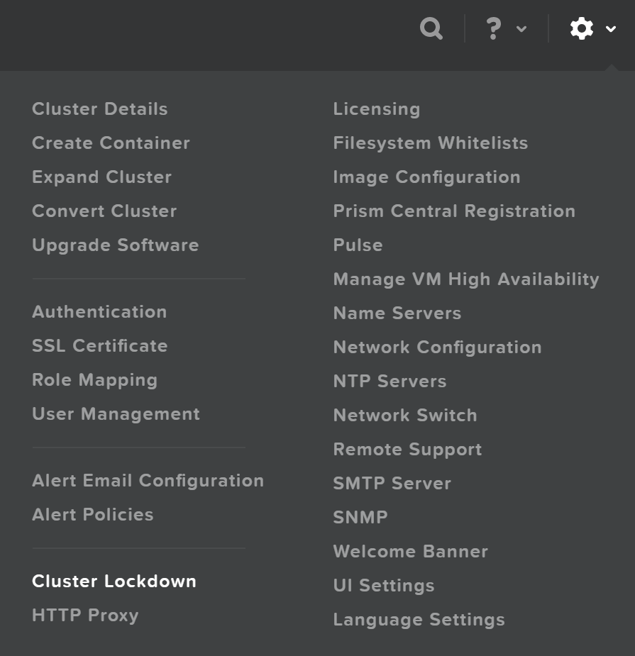
This will show the current configuration and allow you to add/remove SSH keys for access:
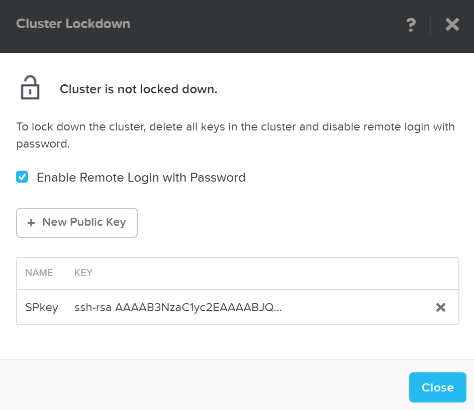
To add a new key click on the 'New Public Key' button and enter the public key details:
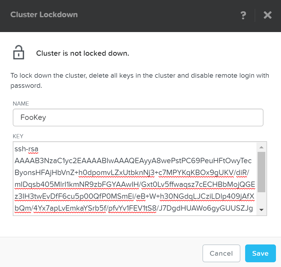
Note
Working with SSH keys
To generate a SSH key, run the following command:
ssh-keygen -t rsa -b 2048
This will generate the key pair which creates to files:
- id_rsa (private key)
- id_rsa.pub (public key - this one is used when adding a key to the cluster)
Once you've added some key(s) and have validated access with them, you can disable password based login, by un-checking 'Enable Remote Login with Password.' A popup will appear to confirm the action, click 'Ok' to proceed with lockdown.
Data Encryption
Nutanix provides data-at-rest encryption leveraging FIPS-140-2 Level-2 validated self-encrypting drives (SED) and an exernal key management server (KMS). Communication with the KMS leverages standard protocols including KMIP and TCG. Example KMS servers include Vormetric, SafeNet, etc.
The figure shows a high-level overview of the architecture:
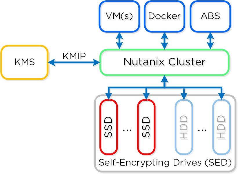
SED encryption works by splitting the storage device into "data bands" which can be in an secured or un-secured state. In the case of Nutanix, the boot and Nutanix Home partitions are trivially encrypted. All data devices and bands are heavily encrypted with big keys to level-2 standards.
When the cluster starts it will call out to the KMS server to get the keys to unlock the drives. In order to ensure security no keys are cached on the cluster. In the event of a cold boot and IPMI reset, the node will need to make a call back to the KMS server to unlock the drives. Soft reboots of the CVM will not force this to occur.
Drive Breakdown
In this section, I’ll cover how the various storage devices (SSD / HDD) are broken down, partitioned, and utilized by the Nutanix platform. NOTE: All of the capacities used are in Base2 Gibibyte (GiB) instead of the Base10 Gigabyte (GB). Formatting of the drives with a filesystem and associated overheads has also been taken into account.
SSD Devices
SSD devices store a few key items which are explained in greater detail above:
- Nutanix Home (CVM core)
- Cassandra (metadata storage)
- OpLog (persistent write buffer)
- Unified Cache (SSD cache portion)
- Extent Store (persistent storage)
The following figure shows an example of the storage breakdown for a Nutanix node’s SSD(s):
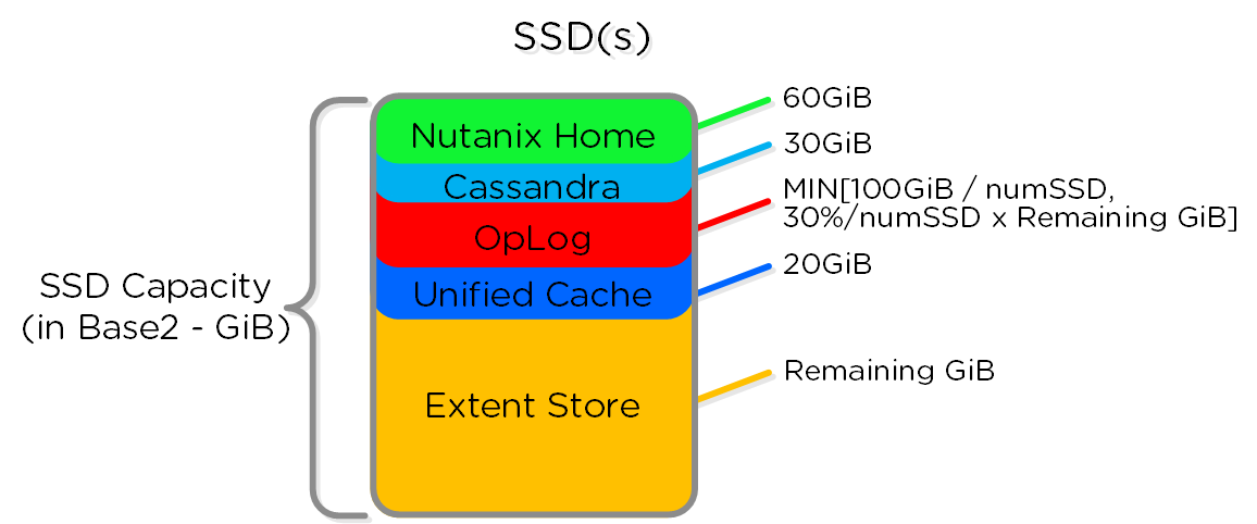
NOTE: The sizing for OpLog is done dynamically as of release 4.0.1 which will allow the extent store portion to grow dynamically. The values used are assuming a completely utilized OpLog. Graphics and proportions aren’t drawn to scale. When evaluating the Remaining GiB capacities, do so from the top down. For example, the Remaining GiB to be used for the OpLog calculation would be after Nutanix Home and Cassandra have been subtracted from the formatted SSD capacity.
Nutanix Home is mirrored across the first two SSDs to ensure availability. Cassandra is on the first SSD by default, and if that SSD fails the CVM will be restarted and Cassandra storage will then be on the 2nd.
Most models ship with 1 or 2 SSDs, however the same construct applies for models shipping with more SSD devices. For example, if we apply this to an example 3060 or 6060 node which has 2 x 400GB SSDs, this would give us 100GiB of OpLog, 40GiB of Unified Cache, and ~440GiB of Extent Store SSD capacity per node.
HDD Devices
Since HDD devices are primarily used for bulk storage, their breakdown is much simpler:
- Curator Reservation (Curator storage)
- Extent Store (persistent storage)
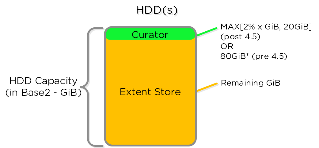
For example, if we apply this to an example 3060 node which has 4 x 1TB HDDs, this would give us 80GiB reserved for Curator and ~3.4TiB of Extent Store HDD capacity per node.
NOTE: the above values are accurate as of 4.0.1 and may vary by release.
Distributed Storage Fabric
The Distributed Storage Fabric (DSF) appears to the hypervisor like any centralized storage array, however all of the I/Os are handled locally to provide the highest performance. More detail on how these nodes form a distributed system can be found in the next section.
Data Structure
The Acropolis Distributed Storage Fabric is composed of the following high-level struct:
Storage Pool
- Key Role: Group of physical devices
- Description: A storage pool is a group of physical storage devices including PCIe SSD, SSD, and HDD devices for the cluster. The storage pool can span multiple Nutanix nodes and is expanded as the cluster scales. In most configurations, only a single storage pool is leveraged.
Container
- Key Role: Group of VMs/files
- Description: A container is a logical segmentation of the Storage Pool and contains a group of VM or files (vDisks). Some configuration options (e.g., RF) are configured at the container level, however are applied at the individual VM/file level. Containers typically have a 1 to 1 mapping with a datastore (in the case of NFS/SMB).
vDisk
- Key Role: vDisk
- Description: A vDisk is any file over 512KB on DSF including .vmdks and VM hard disks. vDisks are composed of extents which are grouped and stored on disk as an extent group.
Note
Maximum DSF vDisk Size
No artificial limits are imposed on the vdisk size on the DSF/stargate side. As of 4.6, the vdisk size is stored as a 64 bit signed integer that stores the size in bytes. This means the theoretical maximum vDisk size can be 2^63-1 or 9E18 (9 Exabytes). Any limits below this value would be due to limitations on the client side, such as the maximum vmdk size on ESXi.
The following figure shows how these map between DSF and the hypervisor:
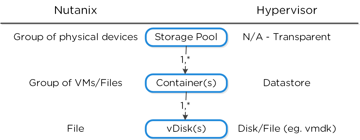
Extent
- Key Role: Logically contiguous data
- Description: An extent is a 1MB piece of logically contiguous data which consists of n number of contiguous blocks (varies depending on guest OS block size). Extents are written/read/modified on a sub-extent basis (aka slice) for granularity and efficiency. An extent’s slice may be trimmed when moving into the cache depending on the amount of data being read/cached.
Extent Group
- Key Role: Physically contiguous stored data
- Description: An extent group is a 1MB or 4MB piece of physically contiguous stored data. This data is stored as a file on the storage device owned by the CVM. Extents are dynamically distributed among extent groups to provide data striping across nodes/disks to improve performance. NOTE: as of 4.0, extent groups can now be either 1MB or 4MB depending on dedupe.
The following figure shows how these structs relate between the various file systems:
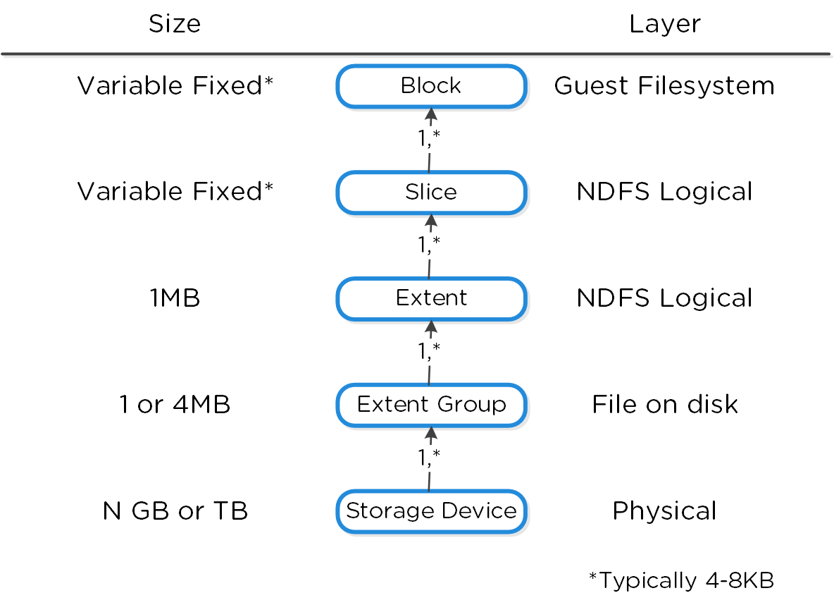
Here is another graphical representation of how these units are related:
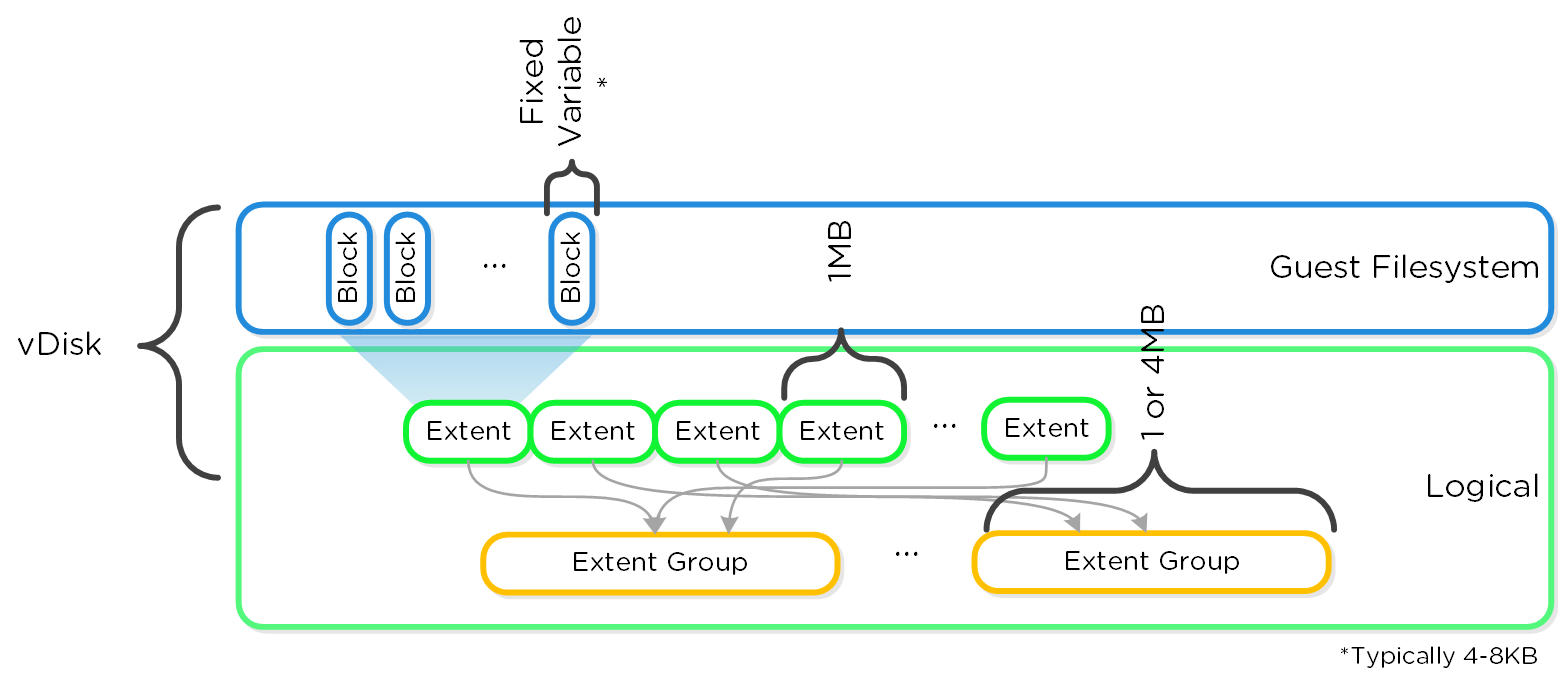
I/O Path and Cache
For a visual explanation, you can watch the following video: LINK
The Nutanix I/O path is composed of the following high-level components:
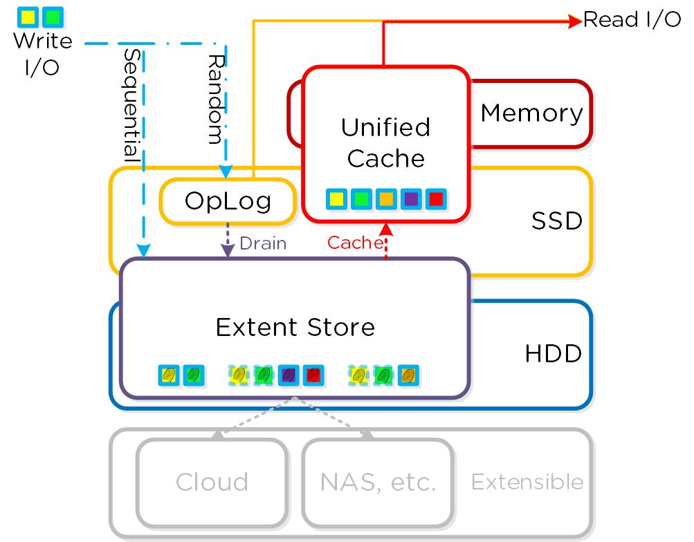
In all-flash node configurations the Extent Store will only consist of SSD devices and no tier ILM will occur as only a single flash tier exists.
OpLog
- Key Role: Persistent write buffer
- Description: The OpLog is similar to a filesystem journal and is built as a staging area to handle bursts of random writes, coalesce them, and then sequentially drain the data to the extent store. Upon a write, the OpLog is synchronously replicated to another n number of CVM’s OpLog before the write is acknowledged for data availability purposes. All CVM OpLogs partake in the replication and are dynamically chosen based upon load. The OpLog is stored on the SSD tier on the CVM to provide extremely fast write I/O performance, especially for random I/O workloads. For sequential workloads, the OpLog is bypassed and the writes go directly to the extent store. If data is currently sitting in the OpLog and has not been drained, all read requests will be directly fulfilled from the OpLog until they have been drained, where they would then be served by the extent store/unified cache. For containers where fingerprinting (aka Dedupe) has been enabled, all write I/Os will be fingerprinted using a hashing scheme allowing them to be deduplicated based upon fingerprint in the unified cache.
Note
Per-vDisk OpLog Sizing
The OpLog is a shared resource, however allocation is done on a per-vDisk basis to ensure each vDisk has an equal opportunity to leverage. This is implemented through a per-vDisk OpLog limit (max amount of data per-vDisk in the OpLog). VMs with multiple vDisk(s) will be able to leverage the per-vDisk limit times the number of disk(s).
The per-vDisk OpLog limit is currently 6GB (as of 4.6), up from 2GB in prior versions.
This is controlled by the following Gflag: vdisk_distributed_oplog_max_dirty_MB.
Extent Store
- Key Role: Persistent data storage
- Description: The Extent Store is the persistent bulk storage of DSF and spans SSD and HDD and is extensible to facilitate additional devices/tiers. Data entering the extent store is either being A) drained from the OpLog or B) is sequential in nature and has bypassed the OpLog directly. Nutanix ILM will determine tier placement dynamically based upon I/O patterns and will move data between tiers.
Note
Sequential Write Characterization
Write IO is deemed as sequential when there is more than 1.5MB of outstanding write IO to a vDisk (as of 4.6). IOs meeting this will bypass the OpLog and go directly to the Extent Store since they are already large chunks of aligned data and won't benefit from coalescing.
This is controlled by the following Gflag: vdisk_distributed_oplog_skip_min_outstanding_write_bytes.
All other IOs, including those which can be large (e.g. >64K) will still be handled by the OpLog.
Unified Cache
- Key Role: Dynamic read cache
- Description: The Unified Cache is a deduplicated read cache which spans both the CVM’s memory and SSD. Upon a read request of data not in the cache (or based upon a particular fingerprint), the data will be placed into the single-touch pool of the Unified Cache which completely sits in memory, where it will use LRU until it is evicted from the cache. Any subsequent read request will “move” (no data is actually moved, just cache metadata) the data into the memory portion of the multi-touch pool, which consists of both memory and SSD. From here there are two LRU cycles, one for the in-memory piece upon which eviction will move the data to the SSD section of the multi-touch pool where a new LRU counter is assigned. Any read request for data in the multi-touch pool will cause the data to go to the peak of the multi-touch pool where it will be given a new LRU counter.
The following figure shows a high-level overview of the Unified Cache:
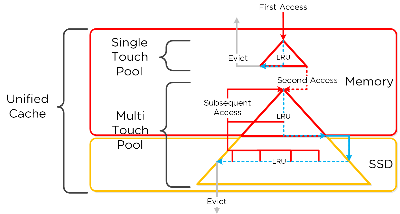
Note
Cache Granularity and Logic
Data is brought into the cache at a 4K granularity and all caching is done real-time (e.g. no delay or batch process data to pull data into the cache).
Each CVM has its own local cache that it manages for the vDisk(s) it is hosting (e.g. VM(s) running on the same node). When a vDisk is cloned (e.g. new clones, snapshots, etc.) each new vDisk has its own block map and the original vDisk is marked as immutable. This allows us to ensure that each CVM can have it's own cached copy of the base vDisk with cache coherency.
In the event of an overwrite, that will be re-directed to a new extent in the VM's own block map. This ensures that there will not be any cache corruption.
Extent Cache
- Key Role: In-memory read cache
- Description: The Extent Cache is an in-memory read cache that is completely in the CVM’s memory. This will store non-fingerprinted extents for containers where fingerprinting and deduplication are disabled. As of version 3.5, this is separate from the Unified Cache, however these are merged in 4.5 with the unified cache.
Scalable Metadata
For a visual explanation, you can watch the following video: LINK
Metadata is at the core of any intelligent system and is even more critical for any filesystem or storage array. In terms of DSF, there are a few key structs that are critical for its success: it has to be right 100% of the time (known as “strictly consistent”), it has to be scalable, and it has to perform at massive scale. As mentioned in the architecture section above, DSF utilizes a “ring-like” structure as a key-value store which stores essential metadata as well as other platform data (e.g., stats, etc.). In order to ensure metadata availability and redundancy a RF is utilized among an odd amount of nodes (e.g., 3, 5, etc.). Upon a metadata write or update, the row is written to a node in the ring and then replicated to n number of peers (where n is dependent on cluster size). A majority of nodes must agree before anything is committed, which is enforced using the Paxos algorithm. This ensures strict consistency for all data and metadata stored as part of the platform.
The following figure shows an example of a metadata insert/update for a 4 node cluster:
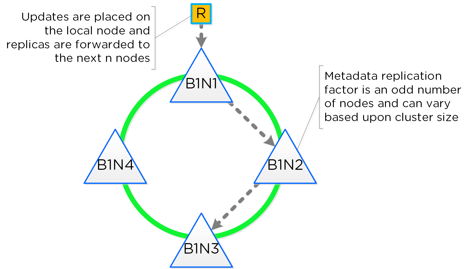
Performance at scale is also another important struct for DSF metadata. Contrary to traditional dual-controller or “master” models, each Nutanix node is responsible for a subset of the overall platform’s metadata. This eliminates the traditional bottlenecks by allowing metadata to be served and manipulated by all nodes in the cluster. A consistent hashing scheme is utilized to minimize the redistribution of keys during cluster size modifications (also known as “add/remove node”) When the cluster scales (e.g., from 4 to 8 nodes), the nodes are inserted throughout the ring between nodes for “block awareness” and reliability.
The following figure shows an example of the metadata “ring” and how it scales:
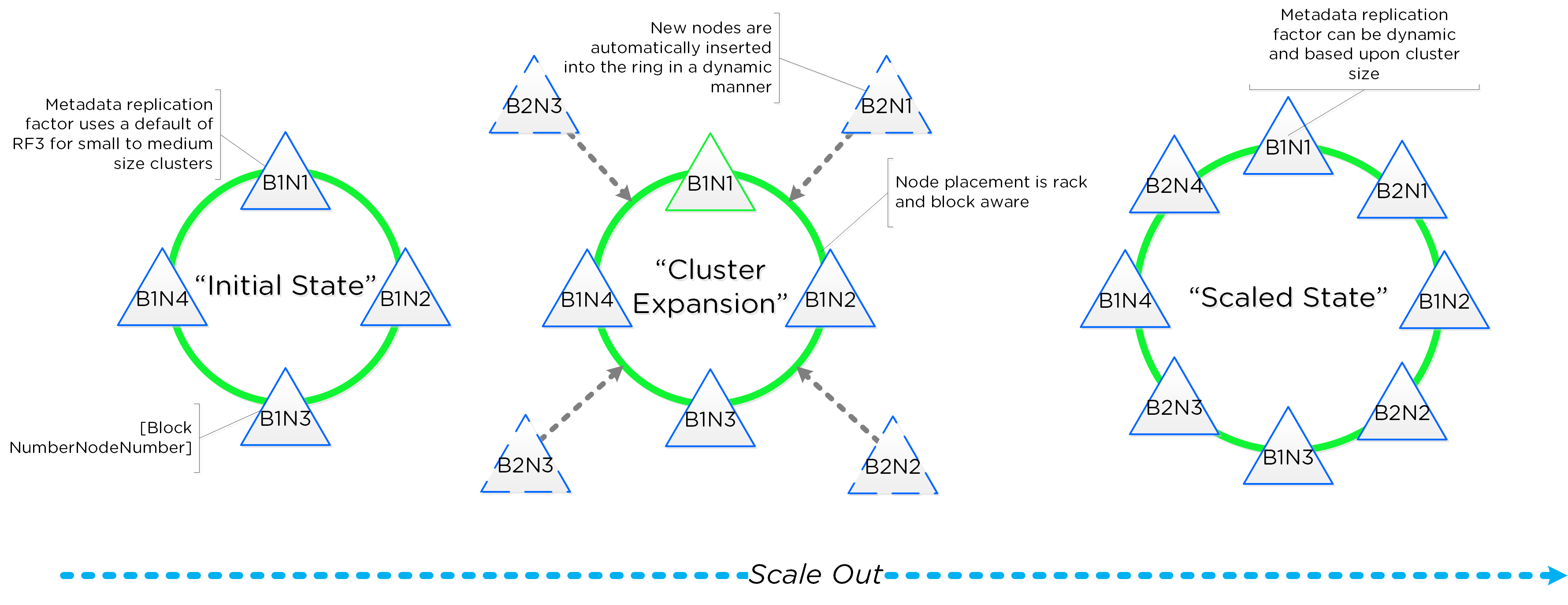
Data Protection
For a visual explanation, you can watch the following video: LINK
The Nutanix platform currently uses a resiliency factor, also known as a replication factor (RF), and checksum to ensure data redundancy and availability in the case of a node or disk failure or corruption. As explained above, the OpLog acts as a staging area to absorb incoming writes onto a low-latency SSD tier. Upon being written to the local OpLog, the data is synchronously replicated to another one or two Nutanix CVM’s OpLog (dependent on RF) before being acknowledged (Ack) as a successful write to the host. This ensures that the data exists in at least two or three independent locations and is fault tolerant. NOTE: For RF3, a minimum of 5 nodes is required since metadata will be RF5.
Data RF is configured via Prism and is done at the container level. All nodes participate in OpLog replication to eliminate any “hot nodes”, ensuring linear performance at scale. While the data is being written, a checksum is computed and stored as part of its metadata. Data is then asynchronously drained to the extent store where the RF is implicitly maintained. In the case of a node or disk failure, the data is then re-replicated among all nodes in the cluster to maintain the RF. Any time the data is read, the checksum is computed to ensure the data is valid. In the event where the checksum and data don’t match, the replica of the data will be read and will replace the non-valid copy.
Data is also consistently monitored to ensure integrity even when active I/O isn't occurring. Stargate's scrubber operation will consistently scan through extent groups and perform checksum validation when disks aren't heavily utilized. This protects against things like bit rot or corrupted sectors.
The following figure shows an example of what this logically looks like:
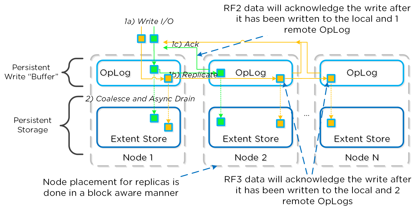
Availability Domains
For a visual explanation, you can watch the following video: LINK
Availability Domains (aka node/block/rack awareness) is a key struct for distributed systems to abide by for determining component and data placement. DSF is currently node and block aware, however this will increase to rack aware as supported cluster sizes grow in the future. Nutanix refers to a “block” as the chassis which contains either one, two, or four server “nodes”. NOTE: A minimum of 3 blocks must be utilized for block awareness to be activated, otherwise node awareness will be defaulted to.
It is recommended to utilized uniformly populated blocks to ensure block awareness is enabled. Common scenarios and the awareness level utilized can be found at the bottom of this section. The 3-block requirement is due to ensure quorum. For example, a 3450 would be a block which holds 4 nodes. The reason for distributing roles or data across blocks is to ensure if a block fails or needs maintenance the system can continue to run without interruption. NOTE: Within a block, the redundant PSU and fans are the only shared components Awareness can be broken into a few key focus areas:
- Data (The VM data)
- Metadata (Cassandra)
- Configuration Data (Zookeeper)
Data
With DSF, data replicas will be written to other blocks in the cluster to ensure that in the case of a block failure or planned downtime, the data remains available. This is true for both RF2 and RF3 scenarios, as well as in the case of a block failure. An easy comparison would be “node awareness”, where a replica would need to be replicated to another node which will provide protection in the case of a node failure. Block awareness further enhances this by providing data availability assurances in the case of block outages.
The following figure shows how the replica placement would work in a 3-block deployment:
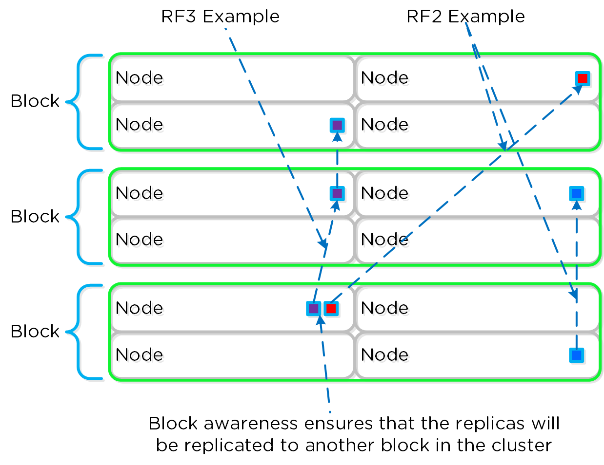
In the case of a block failure, block awareness will be maintained and the re-replicated blocks will be replicated to other blocks within the cluster:
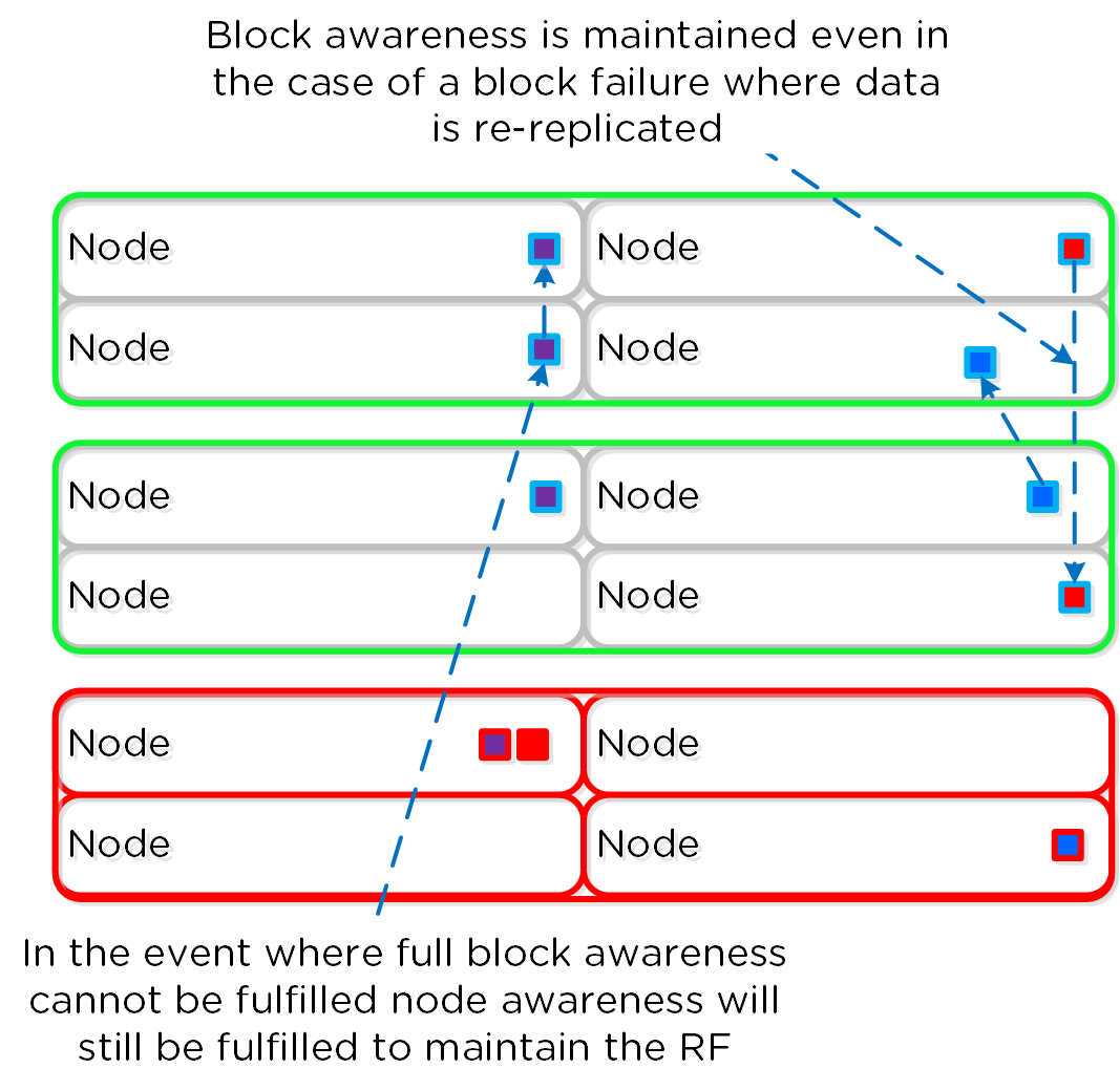
Awareness Conditions and Tolerance
Below we breakdown some common scenarios and the level of tolerance:
| Simultaneous Failure Tolerance | |||
|---|---|---|---|
| Number of Blocks | Awareness Type | Cluster FT1 | Cluster FT2 |
| <3 | NODE | SINGLE NODE | DUAL NODE |
| 3-5 | NODE+BLOCK | SINGLE BLOCK (up to 4 nodes) |
SINGLE BLOCK (up to 4 nodes) |
| 5+ | NODE+BLOCK | SINGLE BLOCK (up to 4 nodes) |
DUAL BLOCK (up to 8 nodes) |
As of Acropolis base software version 4.5 and later block awareness is best effort and doesn't have strict requirements for enabling. This was done to ensure clusters with skewed storage resources (e.g. storage heavy nodes) don't disable the feature. With that stated, it is however still a best practice to have uniform blocks to minimize any storage skew.
Prior to 4.5 the following conditions must be met:
- If SSD or HDD tier variance between blocks is > max variance: NODE awareness
- If SSD and HDD tier variance between blocks is < max variance: BLOCK + NODE awareness
Max tier variance is calculated as: 100 / (RF+1)
- E.g., 33% for RF2 or 25% for RF3
Metadata
As mentioned in the Scalable Metadata section above, Nutanix leverages a heavily modified Cassandra platform to store metadata and other essential information. Cassandra leverages a ring-like structure and replicates to n number of peers within the ring to ensure data consistency and availability.
The following figure shows an example of the Cassandra's ring for a 12-node cluster:
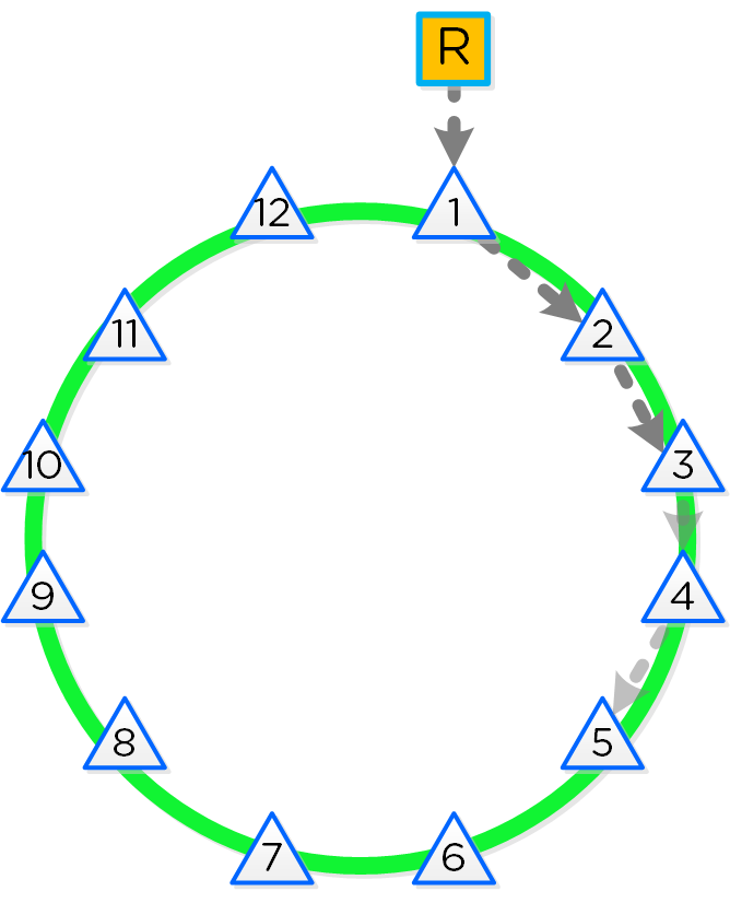
Cassandra peer replication iterates through nodes in a clockwise manner throughout the ring. With block awareness, the peers are distributed among the blocks to ensure no two peers are on the same block.
The following figure shows an example node layout translating the ring above into the block based layout:
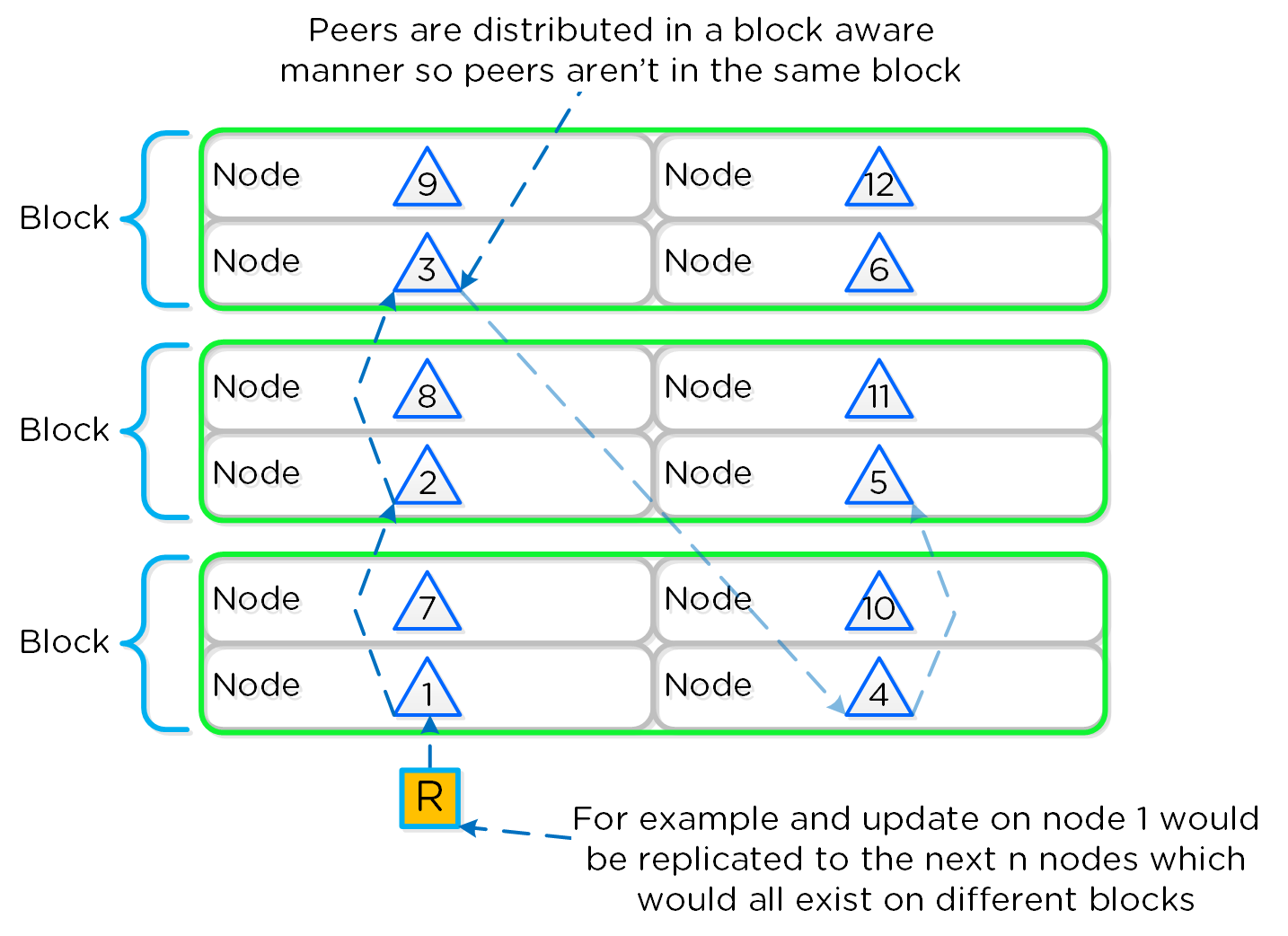
With this block-aware nature, in the event of a block failure there will still be at least two copies of the data (with Metadata RF3 – In larger clusters RF5 can be leveraged).
The following figure shows an example of all of the nodes replication topology to form the ring (yes – it’s a little busy):
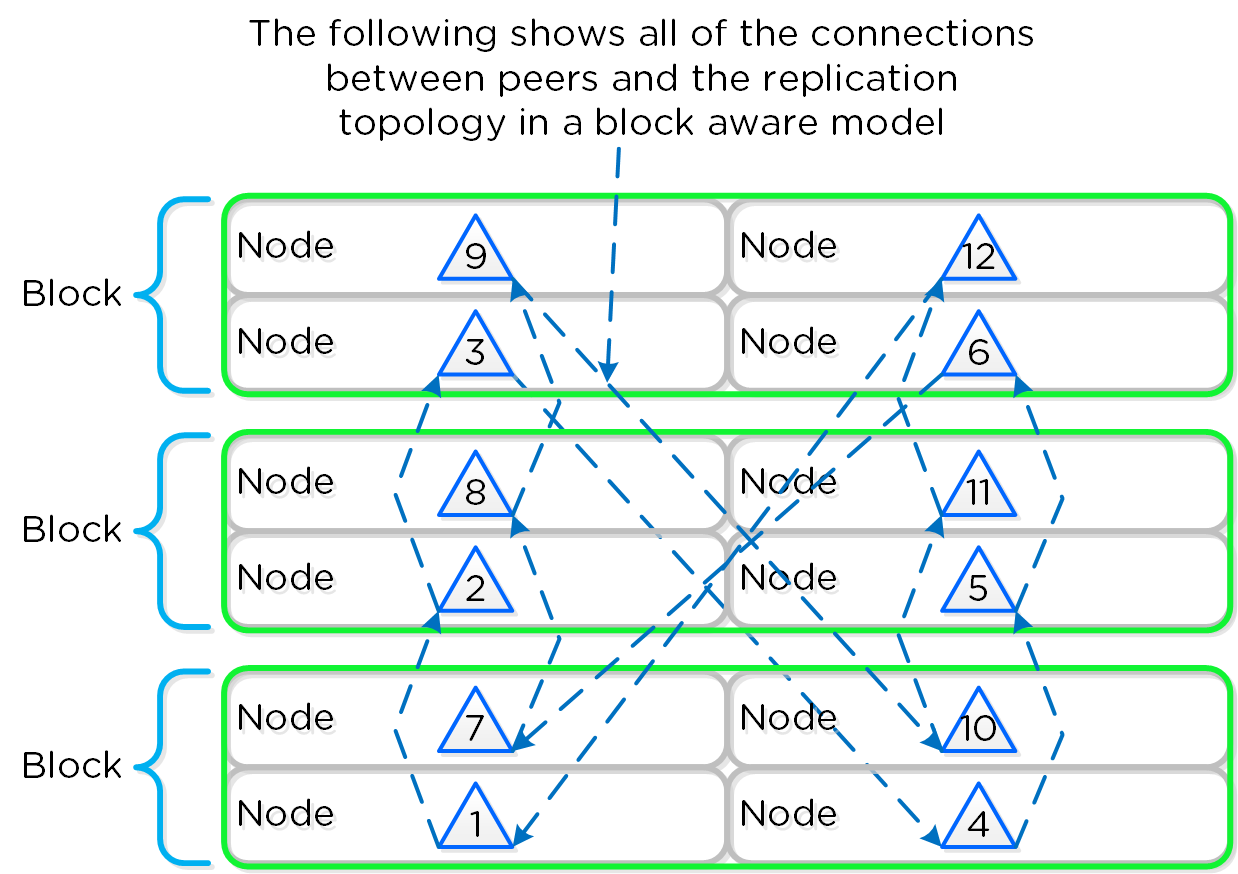
Note
Metadata Awareness Conditions
Below we breakdown some common scenarios and what level of awareness will be utilized:
- FT1 (Data RF2 / Metadata RF3) will be block aware if:
- > 3 blocks
- Let X be the number of nodes in the block with max nodes. Then, the remaining blocks should have at least 2X nodes.
-
Example: 4 blocks with 2,3,4,2 nodes per block respectively.
- The max node block has 4 nodes which means the other 3 blocks should have 2x4 (8) nodes. In this case it WOULD NOT be block aware as the remaining blocks only have 7 nodes.
-
Example: 4 blocks with 3,3,4,3 nodes per block respectively.
- The max node block has 4 nodes which means the other 3 blocks should have 2x4==8 nodes. In this case it WOULD be block aware as the remaining blocks have 9 nodes which is above our minimum.
-
Example: 4 blocks with 2,3,4,2 nodes per block respectively.
- FT2 (Data RF3 / Metadata RF5) will be block aware if:
- > 5 blocks
- Let X be the number of nodes in the block with max nodes. Then, the remaining blocks should have at least 4X nodes.
-
Example: 6 blocks with 2,3,4,2,3,3 nodes per block respectively.
- The max node block has 4 nodes which means the other 3 blocks should have 4x4==16 nodes. In this case it WOULD NOT be block aware as the remaining blocks only have 13 nodes.
-
Example: 6 blocks with 2,4,4,4,4,4 nodes per block respectively.
- The max node block has 4 nodes which means the other 3 blocks should have 4x4==16 nodes. In this case it WOULD be block aware as the remaining blocks have 18 nodes which is above our minimum.
-
Example: 6 blocks with 2,3,4,2,3,3 nodes per block respectively.
Configuration Data
Nutanix leverages Zookeeper to store essential configuration data for the cluster. This role is also distributed in a block-aware manner to ensure availability in the case of a block failure.
The following figure shows an example layout showing 3 Zookeeper nodes distributed in a block-aware manner:
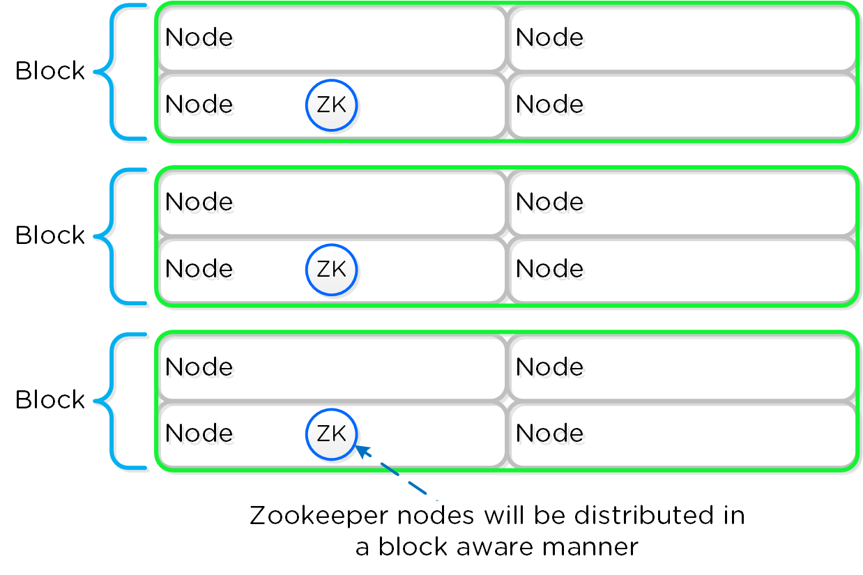
In the event of a block outage, meaning one of the Zookeeper nodes will be gone, the Zookeeper role would be transferred to another node in the cluster as shown below:
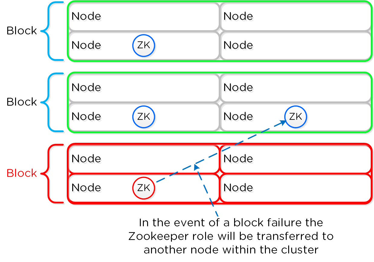
When the block comes back online, the Zookeeper role would be transferred back to maintain block awareness.
NOTE: Prior to 4.5, this migration was not automatic and must be done manually.
Data Path Resiliency
For a visual explanation, you can watch the following video: LINK
Reliability and resiliency are key, if not the most important concepts within DSF or any primary storage platform.
Contrary to traditional architectures which are built around the idea that hardware will be reliable, Nutanix takes a different approach: it expects hardware will eventually fail. By doing so, the system is designed to handle these failures in an elegant and non-disruptive manner.
NOTE: That doesn’t mean the hardware quality isn’t there, just a concept shift. The Nutanix hardware and QA teams undergo an exhaustive qualification and vetting process.
Potential levels of failure
Being a distributed system, DSF is built to handle component, service, and CVM failures, which can be characterized on a few levels:
- Disk Failure
- CVM “Failure”
- Node Failure
Disk Failure
A disk failure can be characterized as just that, a disk which has either been removed, encounters a failure, or one that is not responding or has I/O errors. When Stargate sees I/O errors or the device fails to respond within a certain threshold it will mark the disk offline. Once that has occured Hades will run S.M.A.R.T. and check the status of the device. If the tests pass the disk will be marked online, if they fail it will remain offline. If Stargate marks a disk offline multiple times (currently 3 times in an hour), Hades will stop marking the disk online even if S.M.A.R.T. tests pass.
VM impact:
- HA event: No
- Failed I/Os: No
- Latency: No impact
In the event of a disk failure, a Curator scan (MapReduce Framework) will occur immediately. It will scan the metadata (Cassandra) to find the data previously hosted on the failed disk and the nodes / disks hosting the replicas.
Once it has found that data that needs to be “re-replicated”, it will distribute the replication tasks to the nodes throughout the cluster.
During this process a Drive Self Test (DST) is started for the bad disk and SMART logs are monitored for errors.
An important thing to highlight here is given how Nutanix distributes data and replicas across all nodes / CVMs / disks; all nodes / CVMs / disks will participate in the re-replication.
This substantially reduces the time required for re-protection, as the power of the full cluster can be utilized; the larger the cluster, the faster the re-protection.
CVM “Failure”
A CVM "failure” can be characterized as a CVM power action causing the CVM to be temporarily unavailable. The system is designed to transparently handle these gracefully. In the event of a failure, I/Os will be re-directed to other CVMs within the cluster. The mechanism for this will vary by hypervisor.
The rolling upgrade process actually leverages this capability as it will upgrade one CVM at a time, iterating through the cluster.
VM impact:
- HA event: No
- Failed I/Os: No
- Latency: Potentially higher given I/Os over the network
In the event of a CVM "failure” the I/O which was previously being served from the down CVM, will be forwarded to other CVMs throughout the cluster. ESXi and Hyper-V handle this via a process called CVM Autopathing, which leverages HA.py (like “happy”), where it will modify the routes to forward traffic going to the internal address (192.168.5.2) to the external IP of other CVMs throughout the cluster. This enables the datastore to remain intact, just the CVM responsible for serving the I/Os is remote.
Once the local CVM comes back up and is stable, the route would be removed and the local CVM would take over all new I/Os.
In the case of KVM, iSCSI multi-pathing is leveraged where the primary path is the local CVM and the two other paths would be remote. In the event where the primary path fails, one of the other paths will become active.
Similar to Autopathing with ESXi and Hyper-V, when the local CVM comes back online, it’ll take over as the primary path.
Node Failure
VM Impact:
- HA event: Yes
- Failed I/Os: No
- Latency: No impact
In the event of a node failure, a VM HA event will occur restarting the VMs on other nodes throughout the virtualization cluster. Once restarted, the VMs will continue to perform I/Os as usual which will be handled by their local CVMs.
Similar to the case of a disk failure above, a Curator scan will find the data previously hosted on the node and its respective replicas.
Similar to the disk failure scenario above, the same process will take place to re-protect the data, just for the full node (all associated disks).
In the event where the node remains down for a prolonged period of time (30 minutes as of 4.6), the down CVM will be removed from the metadata ring. It will be joined back into the ring after it has been up and stable for a duration of time.
Note
Pro tip
Data resiliency state will be shown in Prism on the dashboard page.
You can also check data resiliency state via the cli:
# Node status
ncli cluster get-domain-fault-tolerance-status type=node
# Block status
ncli cluster get-domain-fault-tolerance-status type=rackable_unit
These should always be up to date, however to refresh the data you can kick off a Curator partial scan.
Capacity Optimization
The Nutanix platform incorporates a wide range of storage optimization technologies that work in concert to make efficient use of available capacity for any workload. These technologies are intelligent and adaptive to workload characteristics, eliminating the need for manual configuration and fine-tuning.
The following optimizations are leveraged:
- Erasure Coding
- Compression
- Deduplication
More detail on how each of these features can be found in the following sections.
The table describes which optimizations are applicable to workloads a high-level:
| Data Transform | Best suited Application(s) | Comments |
|---|---|---|
| Erasure Coding | Most | Provides higher availability with reduced overheads than traditional RF. No impact to normal write or read I/O performance. Does have some read overhead in the case of a disk / node / block failure where data must be decoded. |
| Inline Compression |
All | No impact to random I/O, helps increase storage tier utilization. Benefits large or sequential I/O performance by reducing data to replicate and read from disk. |
| Offline Compression |
None | Given inline compression will compress only large or sequential writes inline and do random or small I/Os post-process, that should be used instead. |
| Perf Tier Dedup |
P2V/V2V,Hyper-V (ODX),Cross-container clones | Greater cache efficiency for data which wasn't cloned or created using efficient Acropolis clones |
| Capacity Tier Dedup |
Same as perf tier dedup | Benefits of above with reduced overhead on disk |
Erasure Coding
The Nutanix platform leverages a replication factor (RF) for data protection and availability. This method provides the highest degree of availability because it does not require reading from more than one storage location or data re-computation on failure. However, this does come at the cost of storage resources as full copies are required.
To provide a balance between availability while reducing the amount of storage required, DSF provides the ability to encode data using erasure codes (EC).
Similar to the concept of RAID (levels 4, 5, 6, etc.) where parity is calculated, EC encodes a strip of data blocks on different nodes and calculates parity. In the event of a host and/or disk failure, the parity can be leveraged to calculate any missing data blocks (decoding). In the case of DSF, the data block is an extent group and each data block must be on a different node and belong to a different vDisk.
The number of data and parity blocks in a strip is configurable based upon the desired failures to tolerate. The configuration is commonly referred to as the number of <data blocks>/<number of parity blocks>.
For example, “RF2 like” availability (e.g., N+1) could consist of 3 or 4 data blocks and 1 parity block in a strip (e.g., 3/1 or 4/1). “RF3 like” availability (e.g. N+2) could consist of 3 or 4 data blocks and 2 parity blocks in a strip (e.g. 3/2 or 4/2).
Note
Pro tip
You can override the default strip size (4/1 for “RF2 like” or 4/2 for “RF3 like”) via NCLI ‘ctr [create / edit] … erasure-code=<N>/<K>’ where N is the number of data blocks and K is the number of parity blocks. Strip sizes are dynamically sized and integrated with node addition/removal.
The expected overhead can be calculated as <# parity blocks> / <# data blocks>. For example, a 4/1 strip has a 25% overhead or 1.25X compared to the 2X of RF2. A 4/2 strip has a 50% overhead or 1.5X compared to the 3X of RF3.
The following table characterizes the encoded strip sizes and example overheads:
| Cluster Size (nodes) |
EC Strip Size (data/parity blocks) |
EC Overhead (vs. 2X of RF2) |
EC Strip Size (data/parity) |
EC Overhead (vs. 3X of RF3) |
| 4 | 2/1 | 1.5X | N/A | N/A |
| 5 | 3/1 | 1.33X | N/A | N/A |
| 6 | 4/1 | 1.25X | N/A | N/A |
| 7+ | 4/1 | 1.25X | 4/2 | 1.5X |
Note
Pro tip
It is always recommended to have a cluster size which has at least 1 more node than the combined strip size (data + parity) to allow for rebuilding of the strips in the event of a node failure. This eliminates any computation overhead on reads once the strips have been rebuilt (automated via Curator). For example, a 4/1 strip should have at least 6 nodes in the cluster. The previous table follows this best practice.
The encoding is done post-process and leverages the Curator MapReduce framework for task distribution. Since this is a post-process framework, the traditional write I/O path is unaffected.
A normal environment using RF would look like the following:
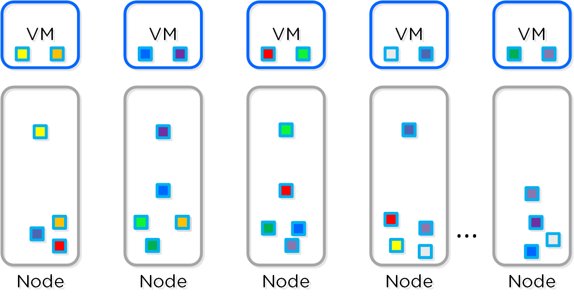
In this scenario, we have a mix of both RF2 and RF3 data whose primary copies are local and replicas are distributed to other nodes throughout the cluster.
When a Curator full scan runs, it will find eligible extent groups which are available to become encoded. Eligible extent groups must be "write-cold" meaning they haven't been written to for awhile. This is controlled with the following Curator Gflag: curator_erasure_code_threshold_seconds. After the eligible candidates are found, the encoding tasks will be distributed and throttled via Chronos.
The following figure shows an example 4/1 and 3/2 strip:
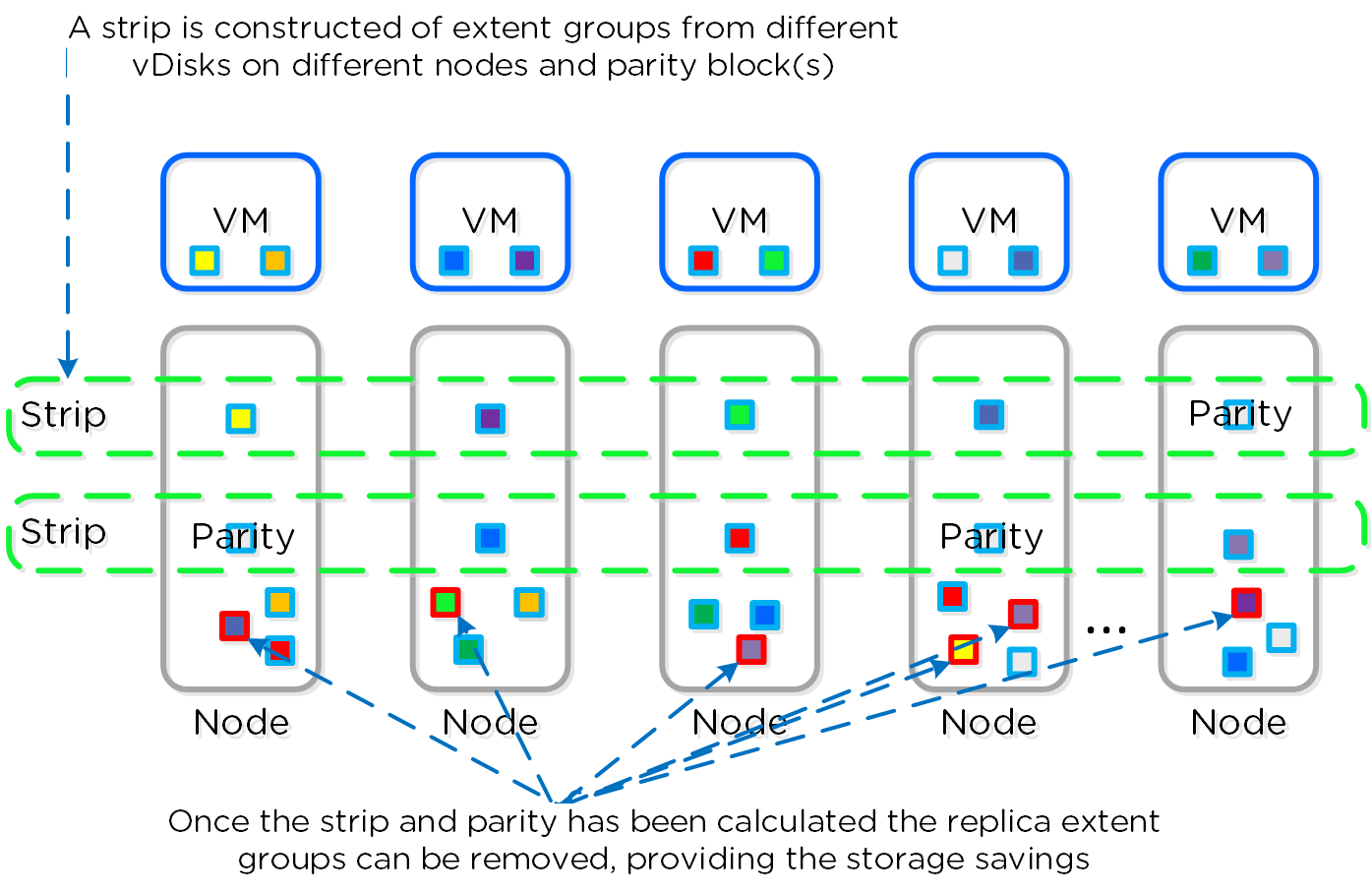
Once the data has been successfully encoded (strips and parity calculation), the replica extent groups are then removed.
The following figure shows the environment after EC has run with the storage savings:
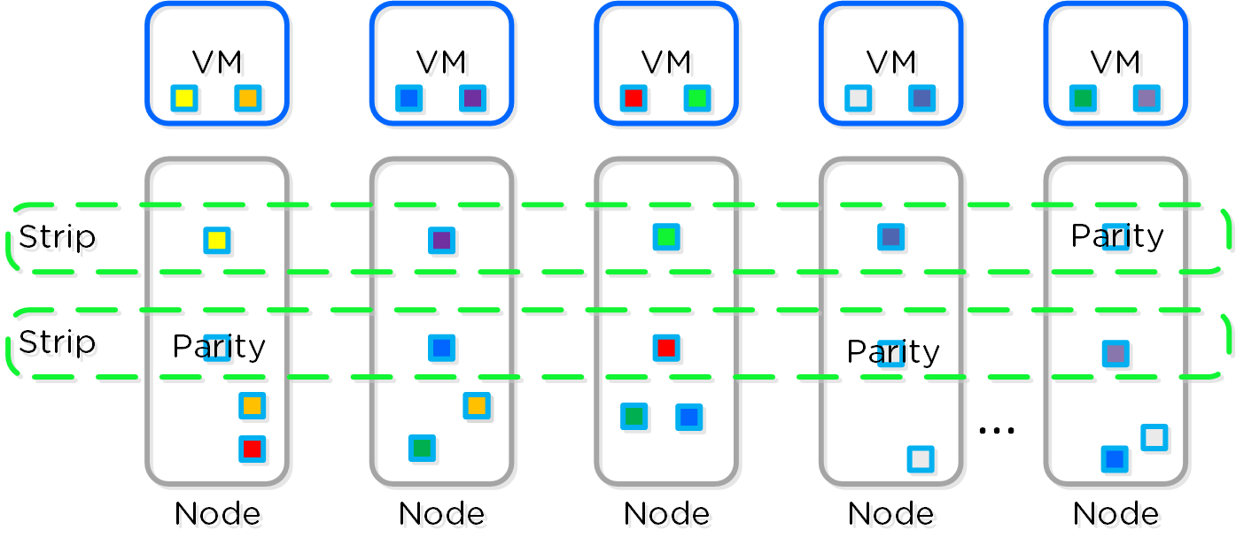
Note
Pro tip
Erasure Coding pairs perfectly with inline compression which will add to the storage savings. I leverage inline compression + EC in my environments.
Compression
For a visual explanation, you can watch the following video: LINK
The Nutanix Capacity Optimization Engine (COE) is responsible for performing data transformations to increase data efficiency on disk. Currently compression is one of the key features of the COE to perform data optimization. DSF provides both inline and offline flavors of compression to best suit the customer’s needs and type of data.
Inline compression will compress sequential streams of data or large I/O sizes (>64K) when written to the Extent Store (SSD + HDD). This includes data draining from OpLog as well as sequential data skipping it.
Note
OpLog Compression
With Asterix the OpLog will now compress all incoming writes >4K that show good compression. This will allow for a more efficient utilization of the OpLog capacity and help drive sustained performance.
When drained from OpLog to the Extent Store the data will be decompressed, aligned and then re-compressed at a 64K aligned unit size.
This feature is on by default and no user configuration is necessary.
Offline compression will initially write the data as normal (in an un-compressed state) and then leverage the Curator framework to compress the data cluster wide. When inline compression is enabled but the I/Os are random in nature, the data will be written un-compressed in the OpLog, coalesced, and then compressed in memory before being written to the Extent Store.
Nutanix leverages LZ4 and LZ4HC for data compression Asterix and beyond. Prior to Asterix the Google Snappy compression library is leveraged which provides good compression ratios with minimal computational overhead and extremely fast compression / decompression rates.
Normal data will be compressed using LZ4 which provides a very good blend between compression and performance. For cold data, LZ4HC will be leveraged to provide an improved compression ratio.
Cold data is characterized into two main categories:
- Regular data: No R/W access for 3 days (Gflag: curator_medium_compress_mutable_data_delay_secs)
- Immutable data (snapshots): No R/W access for 1 day (Gflag: curator_medium_compress_immutable_data_delay_secs)
The following figure shows an example of how inline compression interacts with the DSF write I/O path:
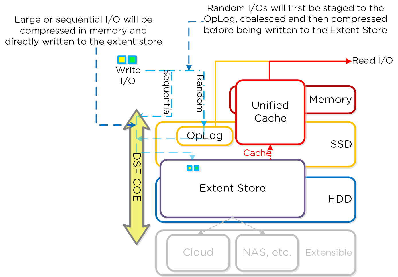
Note
Pro tip
Almost always use inline compression (compression delay = 0) as it will only compress larger / sequential writes and not impact random write performance.
This will also increase the usable size of the SSD tier increasing effective performance and allowing more data to sit in the SSD tier. Also, for larger or sequential data that is written and compressed inline, the replication for RF will be shipping the compressed data, further increasing performance since it is sending less data across the wire.
Inline compression also pairs perfectly with erasure coding.
For offline compression, all new write I/O is written in an un-compressed state and follows the normal DSF I/O path. After the compression delay (configurable) is met, the data is eligible to become compressed. Compression can occur anywhere in the Extent Store. Offline compression uses the Curator MapReduce framework and all nodes will perform compression tasks. Compression tasks will be throttled by Chronos.
The following figure shows an example of how offline compression interacts with the DSF write I/O path:
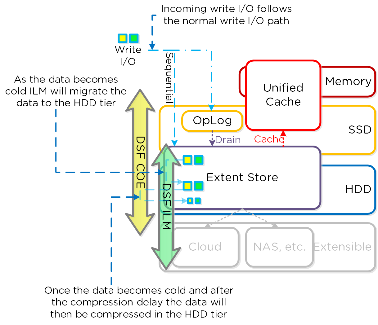
For read I/O, the data is first decompressed in memory and then the I/O is served.
You can view the current compression rates via Prism on the Storage > Dashboard page.
Elastic Dedupe Engine
For a visual explanation, you can watch the following video: LINK
The Elastic Dedupe Engine is a software-based feature of DSF which allows for data deduplication in the capacity (Extent Store) and performance (Unified Cache) tiers. Streams of data are fingerprinted during ingest using a SHA-1 hash at a 16K granularity. This fingerprint is only done on data ingest and is then stored persistently as part of the written block’s metadata. NOTE: Initially a 4K granularity was used for fingerprinting, however after testing 16K offered the best blend of deduplication with reduced metadata overhead. Deduplicated data is pulled into the unified cache at a 4K granularity.
Contrary to traditional approaches which utilize background scans requiring the data to be re-read, Nutanix performs the fingerprint inline on ingest. For duplicate data that can be deduplicated in the capacity tier, the data does not need to be scanned or re-read, essentially duplicate copies can be removed.
To make the metadata overhead more efficient, fingerprint refcounts are monitored to track dedupability. Fingerprints with low refcounts will be discarded to minimize the metadata overhead. To minimize fragmentation full extents will be preferred for capacity tier deduplication.
Note
Pro tip
Use performance tier deduplication on your base images (you can manually fingerprint them using vdisk_manipulator) to take advantage of the unified cache.
Use capacity tier deduplication for P2V / V2V, when using Hyper-V since ODX does a full data copy, or when doing cross-container clones (not usually recommended as a single container is preferred).
In most other cases compression will yield the highest capacity savings and should be used instead.
The following figure shows an example of how the Elastic Dedupe Engine scales and handles local VM I/O requests:
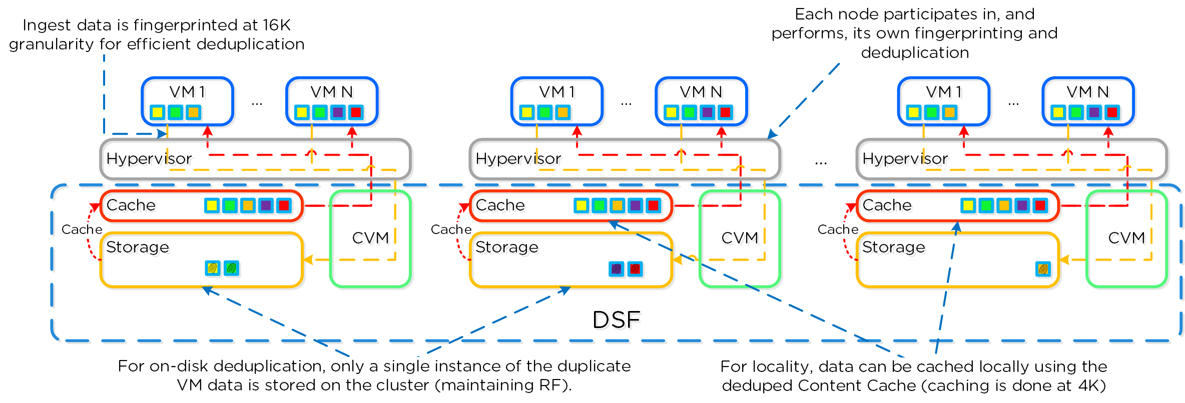
Fingerprinting is done during data ingest of data with an I/O size of 64K or greater (initial I/O or when draining from OpLog). Intel acceleration is leveraged for the SHA-1 computation which accounts for very minimal CPU overhead. In cases where fingerprinting is not done during ingest (e.g., smaller I/O sizes), fingerprinting can be done as a background process. The Elastic Deduplication Engine spans both the capacity tier (Extent Store), but also the performance tier (Unified Cache). As duplicate data is determined, based upon multiple copies of the same fingerprints, a background process will remove the duplicate data using the DSF MapReduce framework (Curator). For data that is being read, the data will be pulled into the DSF Unified Cache which is a multi-tier/pool cache. Any subsequent requests for data having the same fingerprint will be pulled directly from the cache. To learn more about the Unified Cache and pool structure, please refer to the 'Unified Cache' sub-section in the I/O path overview.
Note
Fingerprinted vDisk Offsets
As of 4.6.1 there is no limit and the full vDisk can be fingerprinted / deduped.
Prior to 4.6.1 this was increased to 24GB due to higher metadata efficiencies. Prior to 4.5 only the first 12GB of a vDisk was eligible to be fingerprinted. This was done to maintain a smaller metadata footprint and since the OS is normally the most common data.
The following figure shows an example of how the Elastic Dedupe Engine interacts with the DSF I/O path:
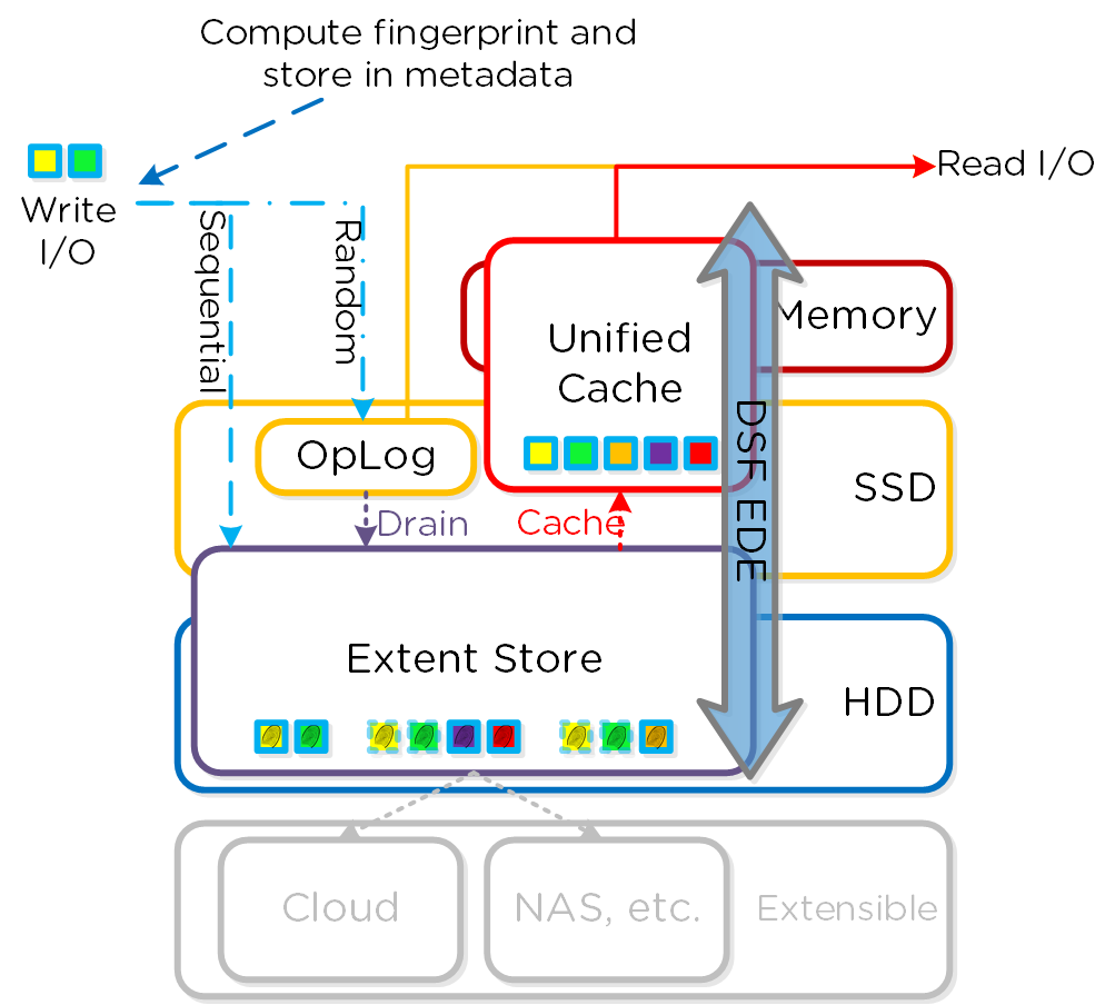
You can view the current deduplication rates via Prism on the Storage > Dashboard page.
Note
Dedup + Compression
As of 4.5 both deduplication and compression can be enabled on the same container. However, unless the data is dedupable (conditions explained earlier in section), stick with compression.
Storage Tiering and Prioritization
The Disk Balancing section above talked about how storage capacity was pooled among all nodes in a Nutanix cluster and that ILM would be used to keep hot data local. A similar concept applies to disk tiering, in which the cluster’s SSD and HDD tiers are cluster-wide and DSF ILM is responsible for triggering data movement events. A local node’s SSD tier is always the highest priority tier for all I/O generated by VMs running on that node, however all of the cluster’s SSD resources are made available to all nodes within the cluster. The SSD tier will always offer the highest performance and is a very important thing to manage for hybrid arrays.
The tier prioritization can be classified at a high-level by the following:
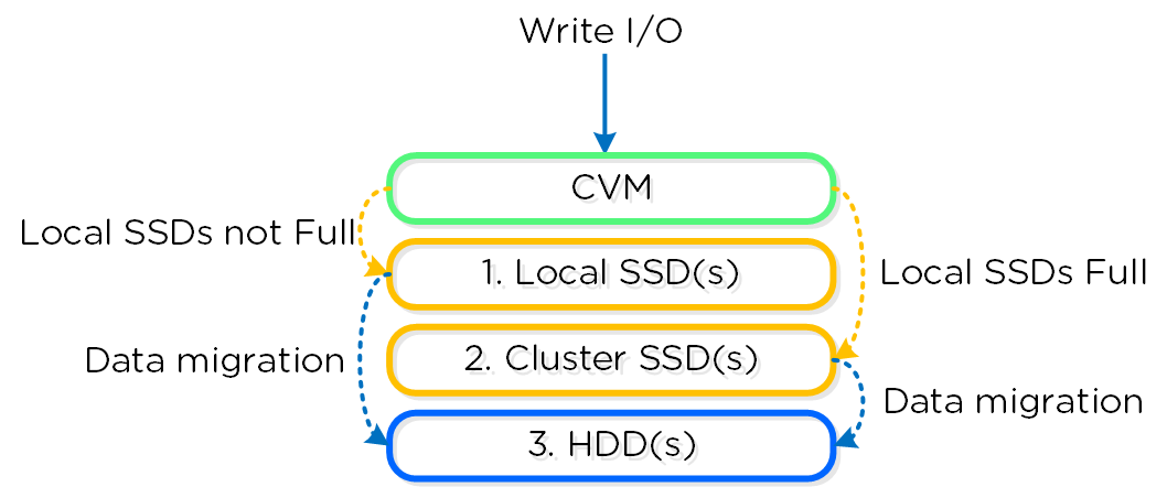
Specific types of resources (e.g. SSD, HDD, etc.) are pooled together and form a cluster wide storage tier. This means that any node within the cluster can leverage the full tier capacity, regardless if it is local or not.
The following figure shows a high level example of what this pooled tiering looks like:
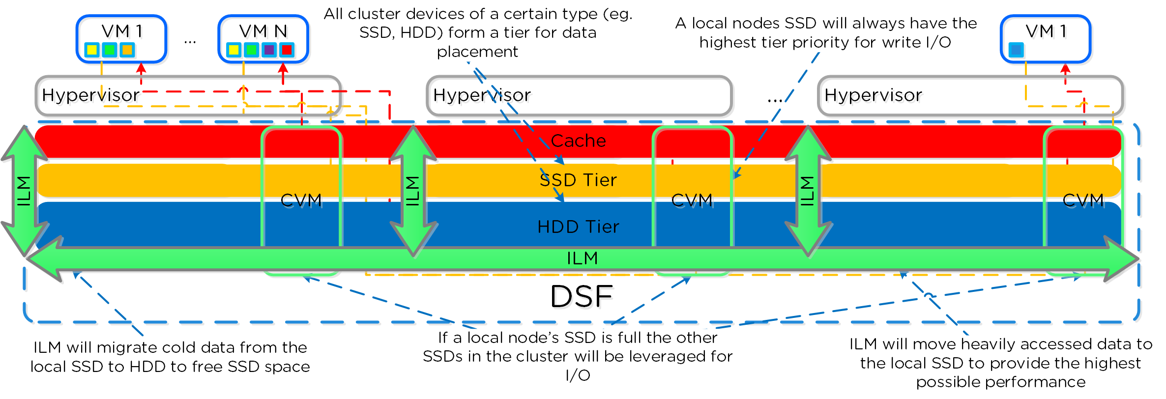
A common question is what happens when a local node’s SSD becomes full? As mentioned in the Disk Balancing section, a key concept is trying to keep uniform utilization of devices within disk tiers. In the case where a local node’s SSD utilization is high, disk balancing will kick in to move the coldest data on the local SSDs to the other SSDs throughout the cluster. This will free up space on the local SSD to allow the local node to write to SSD locally instead of going over the network. A key point to mention is that all CVMs and SSDs are used for this remote I/O to eliminate any potential bottlenecks and remediate some of the hit by performing I/O over the network.
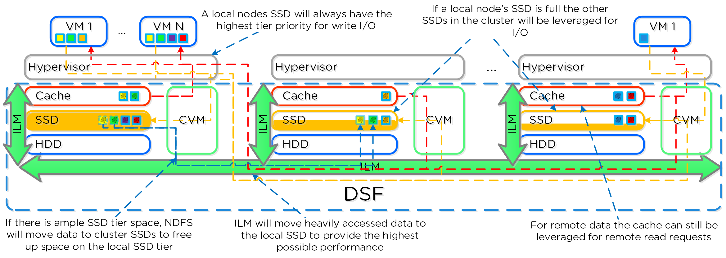
The other case is when the overall tier utilization breaches a specific threshold [curator_tier_usage_ilm_threshold_percent (Default=75)] where DSF ILM will kick in and as part of a Curator job will down-migrate data from the SSD tier to the HDD tier. This will bring utilization within the threshold mentioned above or free up space by the following amount [curator_tier_free_up_percent_by_ilm (Default=15)], whichever is greater. The data for down-migration is chosen using last access time. In the case where the SSD tier utilization is 95%, 20% of the data in the SSD tier will be moved to the HDD tier (95% –> 75%).
However, if the utilization was 80%, only 15% of the data would be moved to the HDD tier using the minimum tier free up amount.
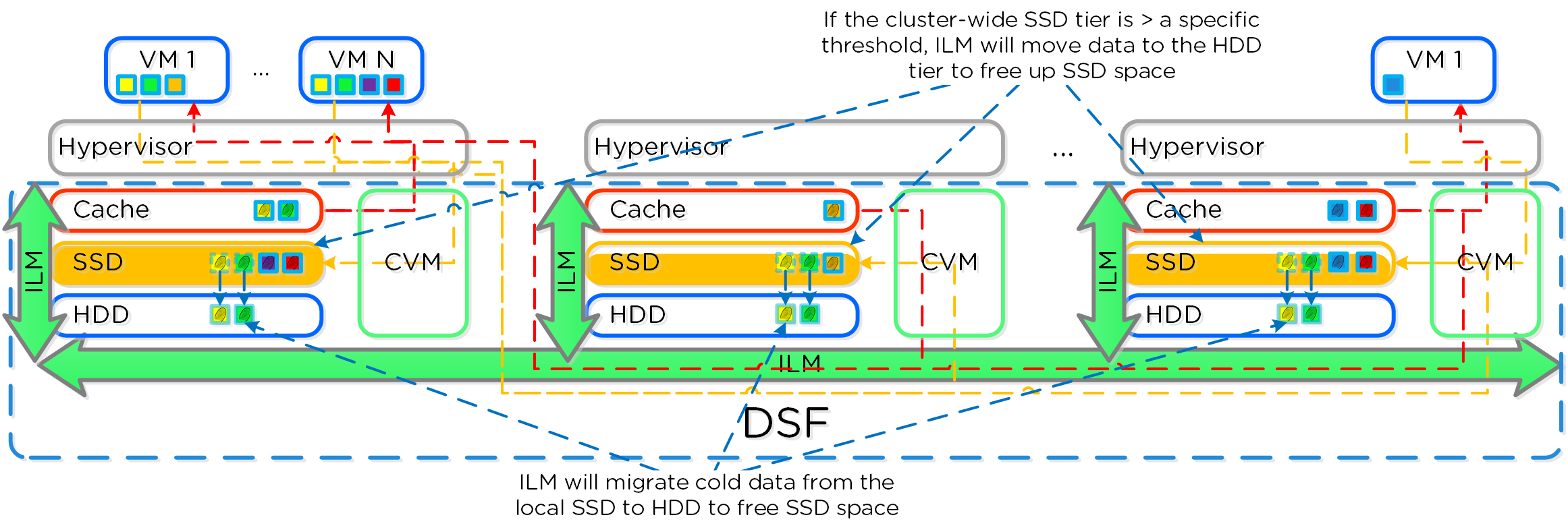
DSF ILM will constantly monitor the I/O patterns and (down/up) migrate data as necessary as well as bring the hottest data local regardless of tier.
Disk Balancing
For a visual explanation, you can watch the following video: LINK
DSF is designed to be a very dynamic platform which can react to various workloads as well as allow heterogeneous node types: compute heavy (3050, etc.) and storage heavy (60X0, etc.) to be mixed in a single cluster. Ensuring uniform distribution of data is an important item when mixing nodes with larger storage capacities. DSF has a native feature, called disk balancing, which is used to ensure uniform distribution of data throughout the cluster. Disk balancing works on a node’s utilization of its local storage capacity and is integrated with DSF ILM. Its goal is to keep utilization uniform among nodes once the utilization has breached a certain threshold.
The following figure shows an example of a mixed cluster (3050 + 6050) in an “unbalanced” state:
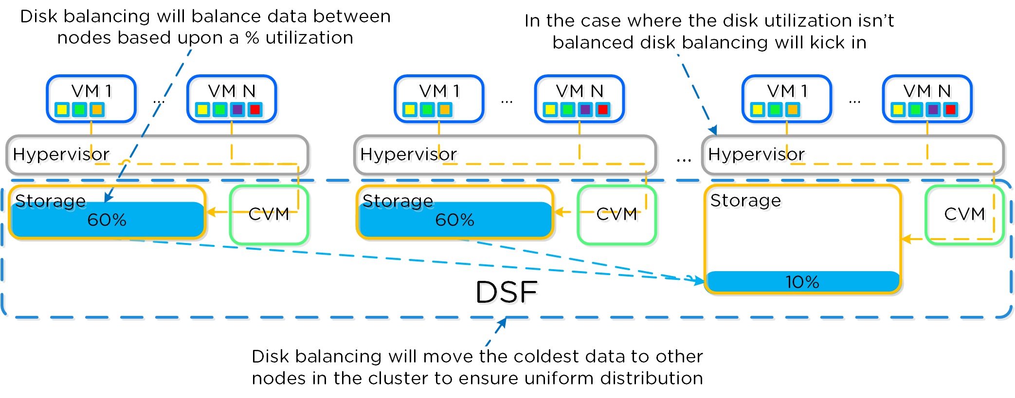
Disk balancing leverages the DSF Curator framework and is run as a scheduled process as well as when a threshold has been breached (e.g., local node capacity utilization > n %). In the case where the data is not balanced, Curator will determine which data needs to be moved and will distribute the tasks to nodes in the cluster. In the case where the node types are homogeneous (e.g., 3050), utilization should be fairly uniform. However, if there are certain VMs running on a node which are writing much more data than others, there can become a skew in the per node capacity utilization. In this case, disk balancing would run and move the coldest data on that node to other nodes in the cluster. In the case where the node types are heterogeneous (e.g., 3050 + 6020/50/70), or where a node may be used in a “storage only” mode (not running any VMs), there will likely be a requirement to move data.
The following figure shows an example the mixed cluster after disk balancing has been run in a “balanced” state:
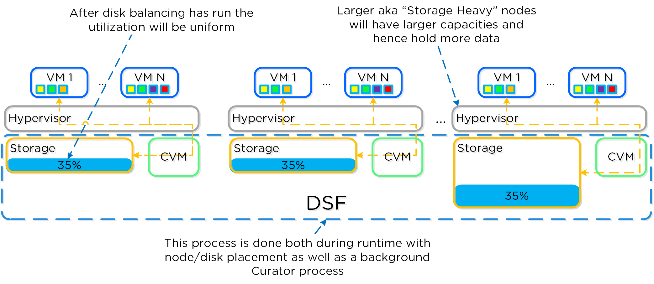
In some scenarios, customers might run some nodes in a “storage-only” state where only the CVM will run on the node whose primary purpose is bulk storage capacity. In this case, the full node's memory can be added to the CVM to provide a much larger read cache.
The following figure shows an example of how a storage only node would look in a mixed cluster with disk balancing moving data to it from the active VM nodes:
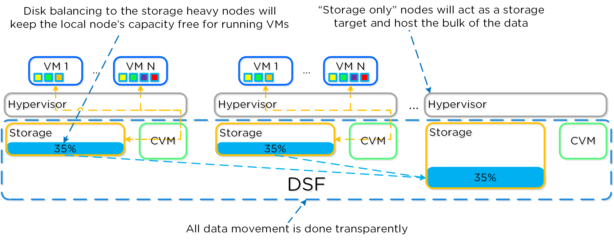
Snapshots and Clones
For a visual explanation, you can watch the following video: LINK
DSF provides native support for offloaded snapshots and clones which can be leveraged via VAAI, ODX, ncli, REST, Prism, etc. Both the snapshots and clones leverage the redirect-on-write algorithm which is the most effective and efficient. As explained in the Data Structure section above, a virtual machine consists of files (vmdk/vhdx) which are vDisks on the Nutanix platform.
A vDisk is composed of extents which are logically contiguous chunks of data, which are stored within extent groups which are physically contiguous data stored as files on the storage devices. When a snapshot or clone is taken, the base vDisk is marked immutable and another vDisk is created as read/write. At this point, both vDisks have the same block map, which is a metadata mapping of the vDisk to its corresponding extents. Contrary to traditional approaches which require traversal of the snapshot chain (which can add read latency), each vDisk has its own block map. This eliminates any of the overhead normally seen by large snapshot chain depths and allows you to take continuous snapshots without any performance impact.
The following figure shows an example of how this works when a snapshot is taken (NOTE: I need to give some credit to NTAP as a base for these diagrams, as I thought their representation was the clearest):
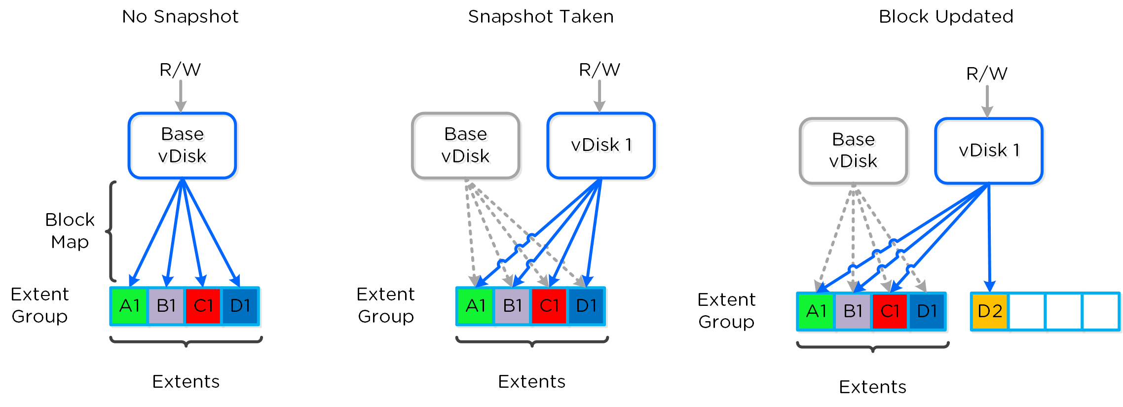
The same method applies when a snapshot or clone of a previously snapped or cloned vDisk is performed:
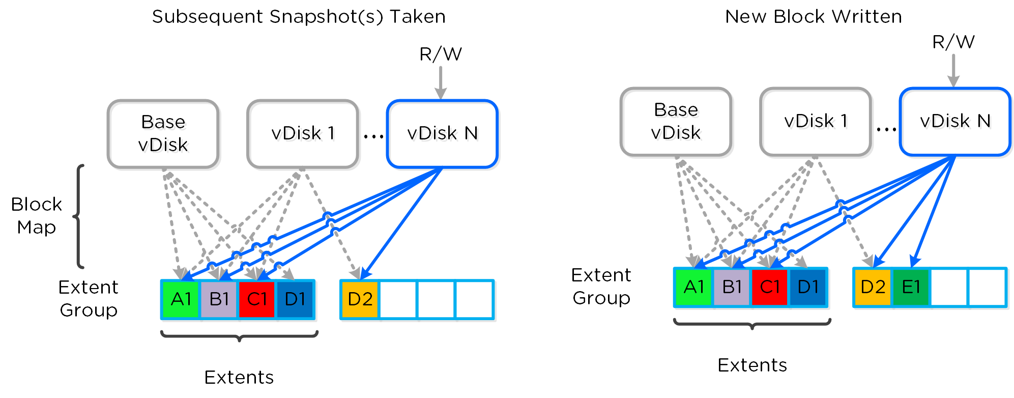
The same methods are used for both snapshots and/or clones of a VM or vDisk(s). When a VM or vDisk is cloned, the current block map is locked and the clones are created. These updates are metadata only, so no I/O actually takes place. The same method applies for clones of clones; essentially the previously cloned VM acts as the “Base vDisk” and upon cloning, that block map is locked and two “clones” are created: one for the VM being cloned and another for the new clone. The is no imposed limit on the maximum number of clones.
They both inherit the prior block map and any new writes/updates would take place on their individual block maps.
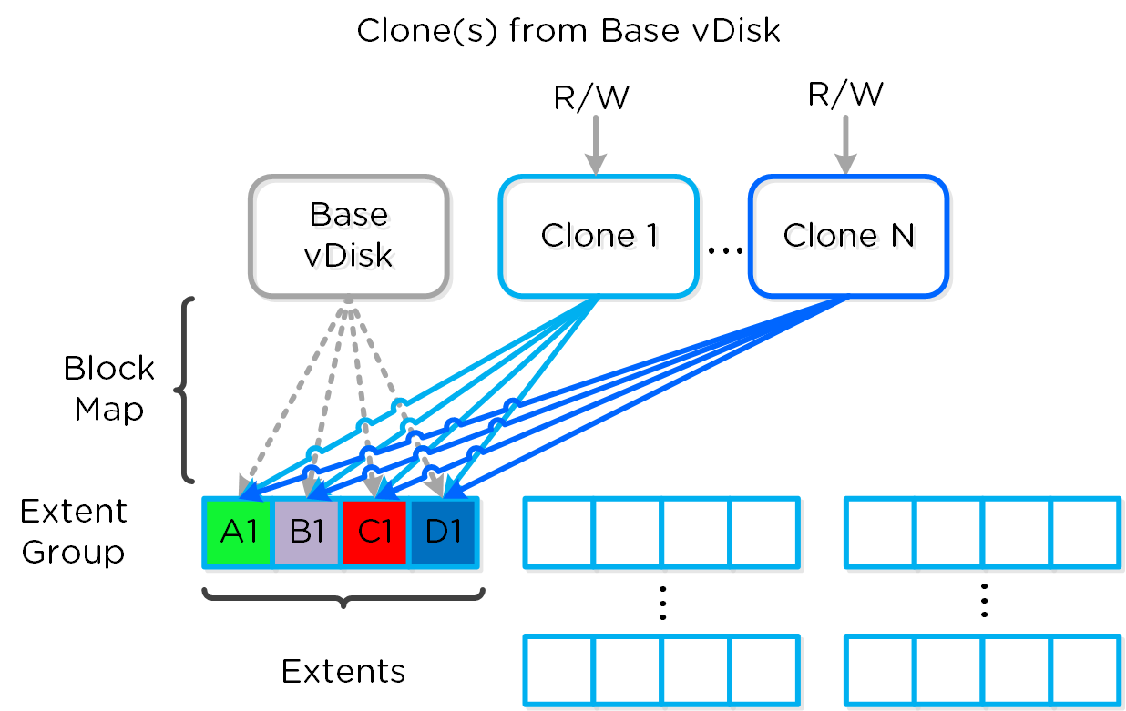
As mentioned previously, each VM/vDisk has its own individual block map. So in the above example, all of the clones from the base VM would now own their block map and any write/update would occur there.
The following figure shows an example of what this looks like:
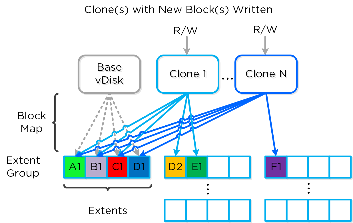
Any subsequent clones or snapshots of a VM/vDisk would cause the original block map to be locked and would create a new one for R/W access.
Networking and I/O
For a visual explanation, you can watch the following video: LINK
The Nutanix platform does not leverage any backplane for inter-node communication and only relies on a standard 10GbE network. All storage I/O for VMs running on a Nutanix node is handled by the hypervisor on a dedicated private network. The I/O request will be handled by the hypervisor, which will then forward the request to the private IP on the local CVM. The CVM will then perform the remote replication with other Nutanix nodes using its external IP over the public 10GbE network. For all read requests, these will be served completely locally in most cases and never touch the 10GbE network. This means that the only traffic touching the public 10GbE network will be DSF remote replication traffic and VM network I/O. There will, however, be cases where the CVM will forward requests to other CVMs in the cluster in the case of a CVM being down or data being remote. Also, cluster-wide tasks, such as disk balancing, will temporarily generate I/O on the 10GbE network.
The following figure shows an example of how the VM’s I/O path interacts with the private and public 10GbE network:
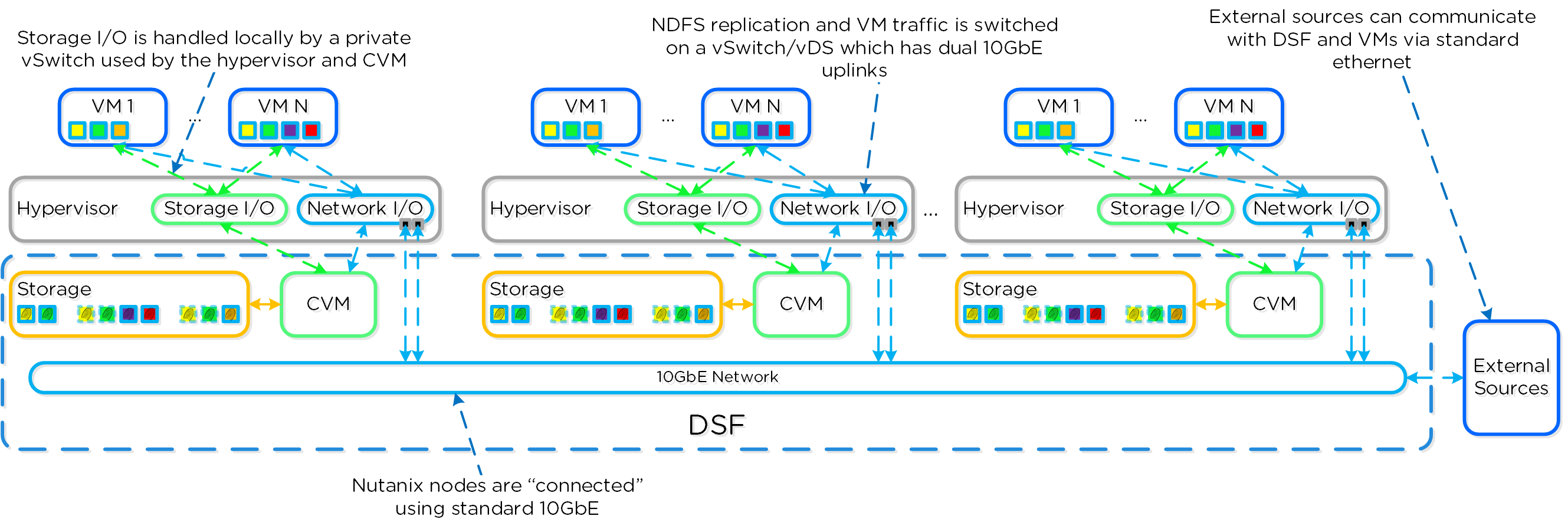
Data Locality
For a visual explanation, you can watch the following video: LINK
Being a converged (compute+storage) platform, I/O and data locality are critical to cluster and VM performance with Nutanix. As explained above in the I/O path, all read/write IOs are served by the local Controller VM (CVM) which is on each hypervisor adjacent to normal VMs. A VM’s data is served locally from the CVM and sits on local disks under the CVM’s control. When a VM is moved from one hypervisor node to another (or during a HA event), the newly migrated VM’s data will be served by the now local CVM. When reading old data (stored on the now remote node/CVM), the I/O will be forwarded by the local CVM to the remote CVM. All write I/Os will occur locally right away. DSF will detect the I/Os are occurring from a different node and will migrate the data locally in the background, allowing for all read I/Os to now be served locally. The data will only be migrated on a read as to not flood the network.
Data locality occurs in two main flavors:
-
Cache Locality
- vDisk data stored locally in the Unified Cache. vDisk extent(s) may be remote to the node.
-
Extent Locality
- vDisk extents local on the same node as the VM
The following figure shows an example of how data will “follow” the VM as it moves between hypervisor nodes:
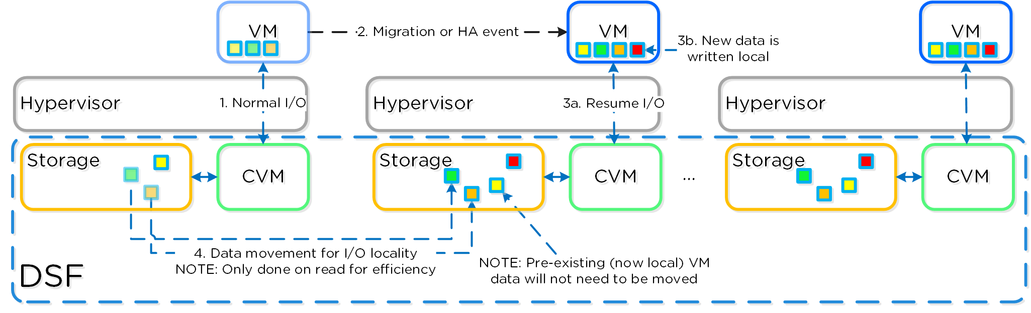
Note
Thresholds for Data Migration
Cache locality occurs in real time and will be determined based upon vDisk ownership. When a vDisk / VM moves from one node to another the "ownership" of those vDisk(s) will transfer to the now local CVM. Once the ownership has transferred the data can be cached locally in the Unified Cache. In the interim the cache will be wherever the ownership is held (the now remote host). The previously hosting Stargate will relinquish the vDisk token when it sees remote I/Os for 300+ seconds at which it will then be taken by the local Stargate. Cache coherence is enforced as ownership is required to cache the vDisk data.
Extent locality is a sampled operation and an extent group will be migrated when the following occurs: "3 touches for random or 10 touches for sequential within a 10 minute window where multiple reads every 10 second sampling count as a single touch".
Shadow Clones
For a visual explanation, you can watch the following video: LINK
The Acropolis Distributed Storage Fabric has a feature called ‘Shadow Clones’, which allows for distributed caching of particular vDisks or VM data which is in a ‘multi-reader’ scenario. A great example of this is during a VDI deployment many ‘linked clones’ will be forwarding read requests to a central master or ‘Base VM’. In the case of VMware View, this is called the replica disk and is read by all linked clones, and in XenDesktop, this is called the MCS Master VM. This will also work in any scenario which may be a multi-reader scenario (e.g., deployment servers, repositories, etc.). Data or I/O locality is critical for the highest possible VM performance and a key struct of DSF.
With Shadow Clones, DSF will monitor vDisk access trends similar to what it does for data locality. However, in the case there are requests occurring from more than two remote CVMs (as well as the local CVM), and all of the requests are read I/O, the vDisk will be marked as immutable. Once the disk has been marked as immutable, the vDisk can then be cached locally by each CVM making read requests to it (aka Shadow Clones of the base vDisk). This will allow VMs on each node to read the Base VM’s vDisk locally. In the case of VDI, this means the replica disk can be cached by each node and all read requests for the base will be served locally. NOTE: The data will only be migrated on a read as to not flood the network and allow for efficient cache utilization. In the case where the Base VM is modified, the Shadow Clones will be dropped and the process will start over. Shadow clones are enabled by default (as of 4.0.2) and can be enabled/disabled using the following NCLI command: ncli cluster edit-params enable-shadow-clones=<true/false>.
The following figure shows an example of how Shadow Clones work and allow for distributed caching:
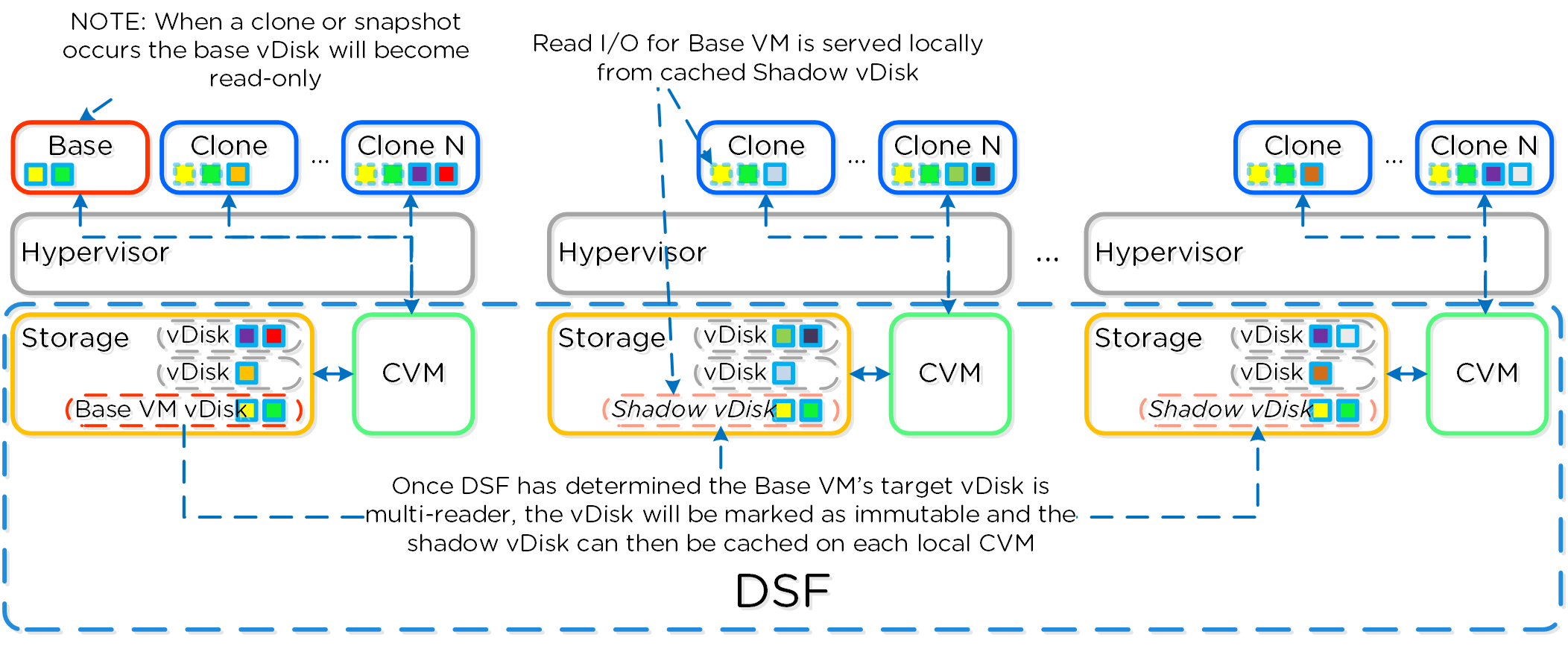
Storage Layers and Monitoring
The Nutanix platform monitors storage at multiple layers throughout the stack, ranging from the VM/Guest OS all the way down to the physical disk devices. Knowing the various tiers and how these relate is important whenever monitoring the solution and allows you to get full visibility of how the ops relate. The following figure shows the various layers of where operations are monitored and the relative granularity which are explained below:
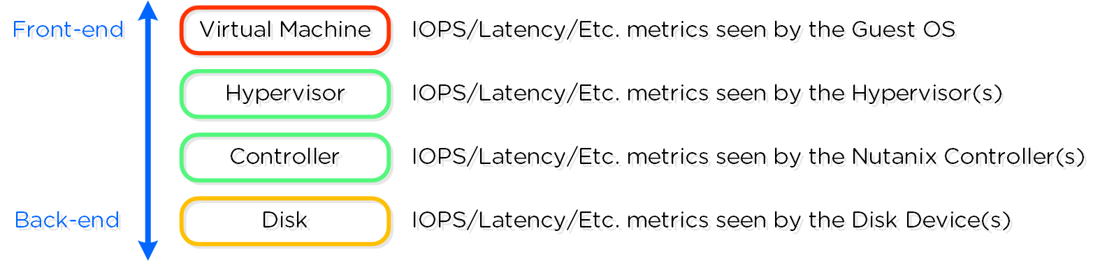
Virtual Machine Layer
- Key Role: Metrics reported by the hypervisor for the VM
- Description: Virtual Machine or guest level metrics are pulled directly from the hypervisor and represent the performance the VM is seeing and is indicative of the I/O performance the application is seeing.
- When to use: When troubleshooting or looking for VM level detail
Hypervisor Layer
- Key Role: Metrics reported by the Hypervisor(s)
- Description: Hypervisor level metrics are pulled directly from the hypervisor and represent the most accurate metrics the hypervisor(s) are seeing. This data can be viewed for one of more hypervisor node(s) or the aggregate cluster. This layer will provide the most accurate data in terms of what performance the platform is seeing and should be leveraged in most cases. In certain scenarios the hypervisor may combine or split operations coming from VMs which can show the difference in metrics reported by the VM and hypervisor. These numbers will also include cache hits served by the Nutanix CVMs.
- When to use: Most common cases as this will provide the most detailed and valuable metrics.
Controller Layer
- Key Role: Metrics reported by the Nutanix Controller(s)
- Description: Controller level metrics are pulled directly from the Nutanix Controller VMs (e.g., Stargate 2009 page) and represent what the Nutanix front-end is seeing from NFS/SMB/iSCSI or any back-end operations (e.g., ILM, disk balancing, etc.). This data can be viewed for one of more Controller VM(s) or the aggregate cluster. The metrics seen by the Controller Layer should normally match those seen by the hypervisor layer, however will include any backend operations (e.g., ILM, disk balancing). These numbers will also include cache hits served by memory. In certain cases, metrics like (IOPS), might not match as the NFS / SMB / iSCSI client might split a large IO into multiple smaller IOPS. However, metrics like bandwidth should match.
- When to use: Similar to the hypervisor layer, can be used to show how much backend operation is taking place.
Disk Layer
- Key Role: Metrics reported by the Disk Device(s)
- Description: Disk level metrics are pulled directly from the physical disk devices (via the CVM) and represent what the back-end is seeing. This includes data hitting the OpLog or Extent Store where an I/O is performed on the disk. This data can be viewed for one of more disk(s), the disk(s) for a particular node, or the aggregate disks in the cluster. In common cases, it is expected that the disk ops should match the number of incoming writes as well as reads not served from the memory portion of the cache. Any reads being served by the memory portion of the cache will not be counted here as the op is not hitting the disk device.
- When to use: When looking to see how many ops are served from cache or hitting the disks.
Note
Metric and Stat Retention
Metrics and time series data is stored locally for 90 days in Prism Element. For Prism Central and Insights, data can be stored indefinitely (assuming capacity is available).
Services
Nutanix Guest Tools (NGT)
Nutanix Guest Tools (NGT) is a software based in-guest agent framework which enables advanced VM management functionality through the Nutanix Platform.
The solution is composed of the NGT installer which is installed on the VMs and the Guest Tools Framework which is used for coordination between the agent and Nutanix platform.
The NGT installer contains the following components:
- Guest Agent Service
- Self-service Restore (SSR) aka File-level Restore (FLR) CLI
- VM Mobility Drivers (VirtIO drivers for AHV)
- VSS Agent and Hardware Provider for Windows VMs
- App Consistent snapshot support for Linux VMs (via scripts to quiesce)
This framework is composed of a few high-level components:
-
Guest Tools Service
- Gateway between the Acropolis and Nutanix services and the Guest Agent. Distributed across CVMs within the cluster with an elected NGT Master which runs on the current Prism Leader (hosting cluster vIP)
-
Guest Agent
- Agent and associated services deployed in the VM's OS as part of the NGT installation process. Handles any local functions (e.g. VSS, Self-service Restore (SSR), etc.) and interacts with the Guest Tools Service.
The figure shows the high-level mapping of the components:
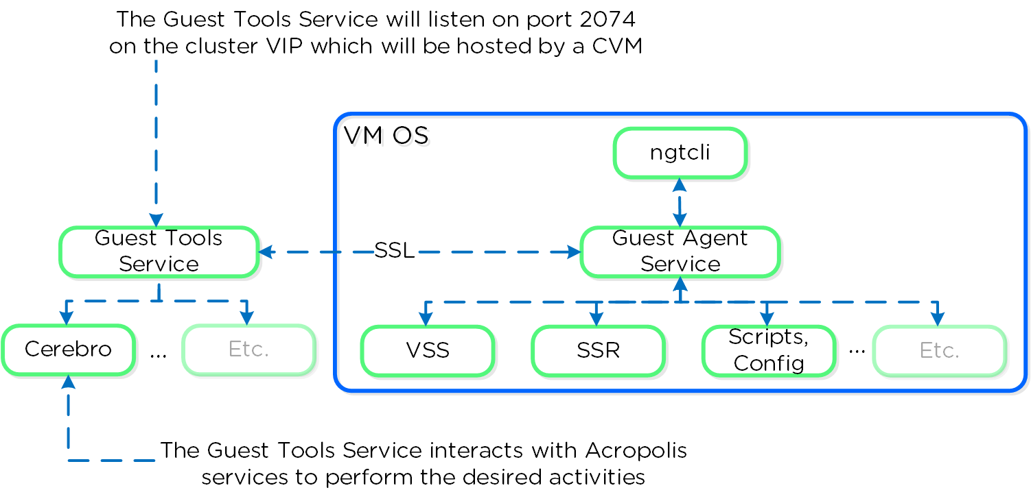
Guest Tools Service
The Guest Tools Service is composed of two main roles:
-
NGT Master
- Handles requests coming from NGT Proxy and interfaces with Acropolis components. A single NGT Master is dynamically elected per cluster; in the event the current master fails a new one will be elected. The service listens internally on port 2073.
-
NGT Proxy
- Runs on every CVM and will forward requests to the NGT Master to perform the desired activity. The current VM activing as the Prism Leader (hosting the VIP) will be the active CVM handling communication from the Guest Agent. Listens externally on port 2074.
Note
Current NGT Master
You can find the IP of the CVM hosting the NGT Master role with the following command (run on any CVM):
nutanix_guest_tools_cli get_master_location
The figure shows the high-level mapping of the roles:
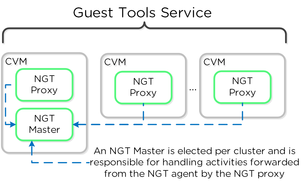
Guest Agent
The Guest Agent is composed of the following high-level components as mentioned prior:
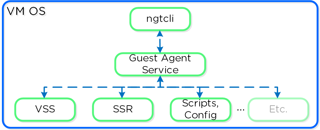
Communication and Security
The Guest Agent Service communicates with Guest Tools Service via the Nutanix Cluster IP using SSL. For deployments where the Nutanix cluster components and UVMs are on a different network (hopefully all), ensure that the following are possible:
- Ensure routed communication from UVM network(s) to Cluster IP OR OR
- Create a firewall rule (and associated NAT) from UVM network(s) allowing communication with the Cluster IP on port 2074 (preferred)
The Guest Tools Service acts as a Certificate Authority (CA) and is responsible for generating certificate pairs for each NGT enabled UVM. This certificate is embedded in to the ISO which is configured for the UVM and used as part of the NGT deployment process. These certificates are installed inside the UVM as part of the installation process.
NGT Agent Installation
NGT Agent installation can be performed via Prism or CLI/Scripts (ncli/REST/PowerShell).
To install NGT via Prism, navigate to the 'VM' page, select a VM to install NGT on and click 'Enable NGT':
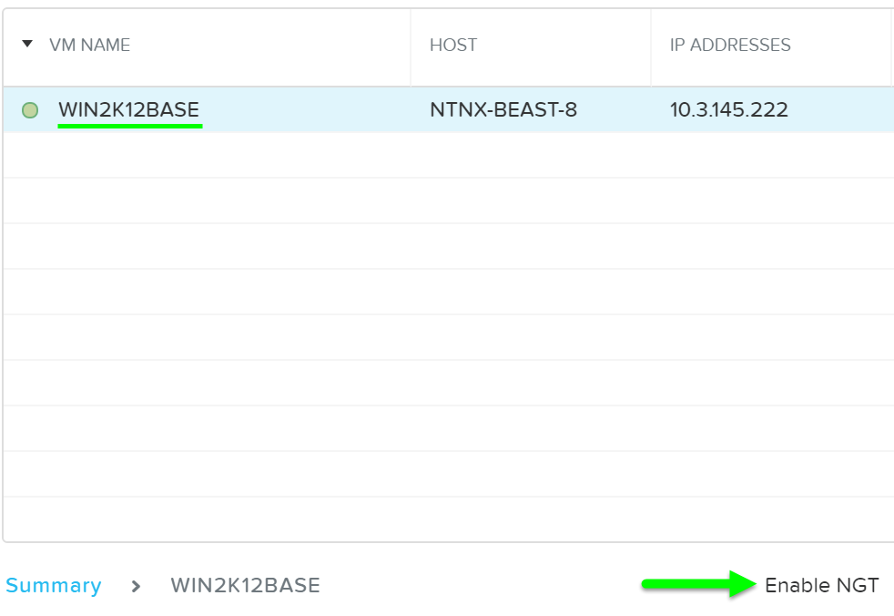
Click 'Yes' at the prompt to continue with NGT installation:

The VM must have a CD-ROM as the generated installer containing the software and unique certificate will be mounted there as shown:
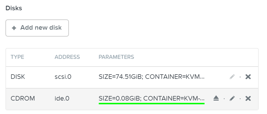
The NGT installer CD-ROM will be visible in the OS:
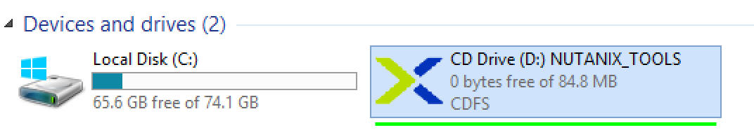
Double click on the CD to begin the installation process.
Note
Silent Installation
You can perform a silent installation of the Nutanix Guest Tools by running the following command (from CD-ROM location):
NutanixGuestTools.exe /quiet /l log.txt ACCEPTEULA=yes
Follow the prompts and accept the licenses to complete the installation:
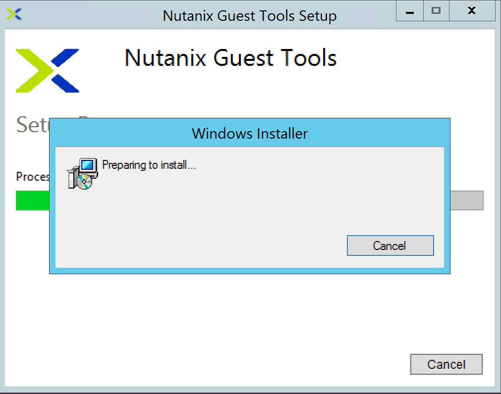
As part of the installation process Python, PyWin and the Nutanix Mobility (cross-hypervisor compatibility) drivers will also be installed.
After the installation has been completed, a reboot will be required.
After successful installation and reboot, you will see the following items visible in 'Programs and Features':
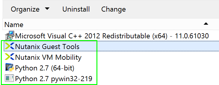
Services for the NGT Agent and VSS Hardware Provider will also be running:
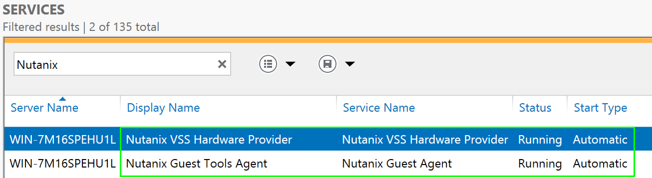
NGT is now installed and can be leveraged.
Note
Bulk NGT Deployment
Rather than installing NGT on each individual VM, it is possible to embed and deploy NGT in your base image.
Follow the following process to leverage NGT inside a base image:
- Install NGT on master VM and ensure communication
- Clone VMs from master VM
-
Mount NGT ISO on each clone (required to get new certificate pair)
- Example: ncli ngt mount vm-id=<CLONE_ID> OR via Prism
- Automated way coming soon :)
- Power on clones
When the cloned VM is booted it will detect the new NGT ISO and copy relevant configuration files and new certificates and will start communicating with the Guest Tools Service.
OS Customization
Nutanix provides native OS customization capabilities leveraging CloudInit and Sysprep. CloudInit is a package which handles bootstrapping of Linux cloud servers. This allows for the early initialization and customization of a Linux instance. Sysprep is a OS customization for Windows.
Some typical uses include:
- Setting Hostname
- Installing packages
- Adding users / key management
- Custom scripts
Supported Configurations
The solution is applicable to Linux guests running on AHV, including versions below (list may be incomplete, refer to documentation for a fully supported list):
-
Hypervisors:
- AHV
-
Operating Systems:
- Linux - most modern distributions
- Windows - most modern distributions
Pre-Requisites
In order for CloudInit to be used the following are necessary:
- CloudInit package must be installed in Linux image
Sysprep is available by default in Windows installations.
Package Installation
CloudInit can be installed (if not already) using the following commands:
Red Hat Based Systems (CentOS, RHEL)
yum -y install CloudInit
Debian Based Systems (Ubuntu)
apt-get -y update; apt-get -y install CloudInit
Sysprep is part of the base Windows installation.
Image Customization
To leverage a custom script for OS customization, a check box and inputs is available in Prism or the REST API. This option is specified during the VM creation or cloning process:
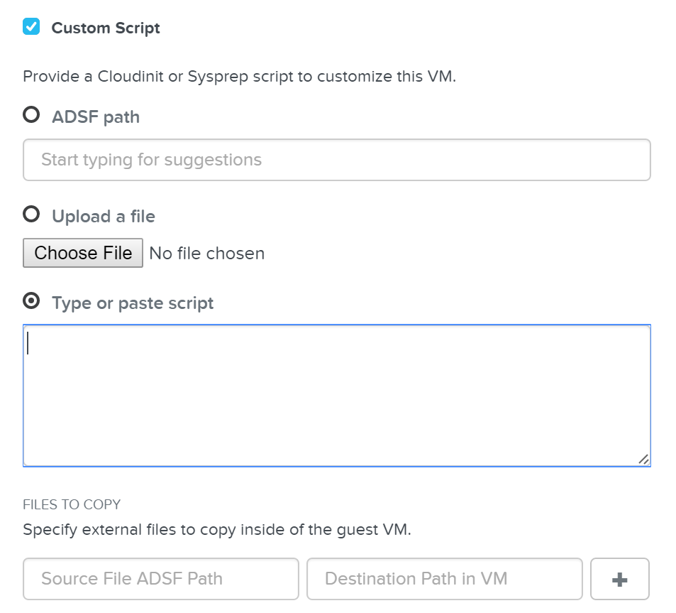
Nutanix has a few options for specifying the custom script path:
-
ADSF Path
- Use a file which has been previously upload to ADSF
-
Upload a file
- Upload a file which will be used
-
Type or paste script
- CloudInit script or Unattend.xml text
Nutanix passes the user data script to CloudInit or Sysprep process during first boot by creating a CD-ROM which contains the script. Once the process is complete we will remove the CD-ROM.
Input formatting
The platform supports a good amount of user data input formats, I've identified a few of the key ones below:
User-Data Script (CloudInit - Linux)
A user-data script is a simple shell script that will be executed very late in the boot process (e.g. "rc.local-like").
The scripts will begin similar to any bash script: "#!".
Below we show an example user-data script:
#!/bin/bash touch /tmp/fooTest mkdir /tmp/barFolder
Include File (CloudInit - Linux)
The include file contains a list of urls (one per line). Each of the URLs will be read and they will be processed similar to any other script.
The scripts will begin with: "#include".
Below we show an example include script:
#include http://s3.amazonaws.com/path/to/script/1 http://s3.amazonaws.com/path/to/script/2
Cloud Config Data (CloudInit - Linux)
The cloud-config input type is the most common and specific to CloudInit.
The scripts will begin with: "#cloud-config"
Below we show an example cloud config data script:
#cloud-config

# Set hostname
hostname: foobar

# Add user(s)
users:
  - name: nutanix
    sudo: ['ALL=(ALL) NOPASSWD:ALL']
    ssh-authorized-keys:
      - ssh-rsa: <PUB KEY>
    lock-passwd: false
    passwd: <PASSWORD>

# Automatically update all of the packages
package_upgrade: true
package_reboot_if_required: true

# Install the LAMP stack
packages:
  - httpd
  - mariadb-server
  - php
  - php-pear
  - php-mysql

# Run Commands after execution
runcmd:
  - systemctl enable httpd
Note
Validating CloudInit Execution
CloudInit log files can be found in /var/log/cloud-init.log and cloud-init-output.log.
Unattend.xml (Sysprep - Windows)
The unattend.xml file is the input file Sysprep uses for image customization on boot, you can read more here: LINK
The scripts will begin with: "<?xml version="1.0" ?>".
Below we show an example unattend.xml file:
<?xml version="1.0" ?>
<unattend xmlns="urn:schemas-microsoft-com:unattend">
   <settings pass="windowsPE">
      <component name="Microsoft-Windows-Setup" publicKeyToken="31bf3856ad364e35"
language="neutral" versionScope="nonSxS" processorArchitecture="x86">
         <WindowsDeploymentServices>
            <Login>
               <WillShowUI>OnError</WillShowUI>
               <Credentials>
                     <Username>username</Username>
                     <Domain>Fabrikam.com</Domain>
                     <Password>my_password</Password>
                  </Credentials>
               </Login>
            <ImageSelection>
               <WillShowUI>OnError</WillShowUI>
               <InstallImage>
                  <ImageName>Windows Vista with Office</ImageName>
                  <ImageGroup>ImageGroup1</ImageGroup>
                  <Filename>Install.wim</Filename>
               </InstallImage>
                  <InstallTo>
                  <DiskID>0</DiskID>
                  <PartitionID>1</PartitionID>
               </InstallTo>
            </ImageSelection>
         </WindowsDeploymentServices>
         <DiskConfiguration>
            <WillShowUI>OnError</WillShowUI>
               <Disk>
                  <DiskID>0</DiskID>
                  <WillWipeDisk>false</WillWipeDisk>
                  <ModifyPartitions>
                     <ModifyPartition>
                        <Order>1</Order>
                        <PartitionID>1</PartitionID>
                        <Letter>C</Letter>
                        <Label>TestOS</Label>
                        <Format>NTFS</Format>
                        <Active>true</Active>
                        <Extend>false</Extend>
                     </ModifyPartition>
                  </ModifyPartitions>
            </Disk>
         </DiskConfiguration>
      </component>
      <component name="Microsoft-Windows-International-Core-WinPE" publicKeyToken="31bf3856ad364e35"
language="neutral" versionScope="nonSxS" processorArchitecture="x86">
         <SetupUILanguage>
            <WillShowUI>OnError</WillShowUI>
            <UILanguage>en-US</UILanguage>
         </SetupUILanguage>
         <UILanguage>en-US</UILanguage>
      </component>
   </settings>
</unattend>
Block Services
The Acropolis Block Services (ABS) feature exposes back-end DSF storage to external consumers (guest OS, physical hosts, containers, etc.) via iSCSI.
This allows any operating system to access DSF and leverage its storage capabilities. In this deployment scenario, the OS is talking directly to Nutanix bypassing any hypervisor.
Core use-cases for Acropolis Block Services:
- Shared Disks
- Oracle RAC, Microsoft Failover Clustering, etc.
- Disks as first-class entities
- Where execution contexts are ephemeral and data is critical
- Containers, OpenStack, etc.
- Guest-initiated iSCSI
- Bare-metal consumers
- Exchange on vSphere (for Microsoft Support)
Qualified Operating Systems
The solution is iSCSI spec compliant, the qualified operating systems are just those of which have been validated by QA.
- Microsoft Windows Server 2008 R2, 2012 R2
- Redhat Enterprise Linux 6.0+
Block Services Constructs
The following entities compose Acropolis Block Services:
- Data Services IP: Cluster wide IP address used for iSCSI login requests (Introduced in 4.7)
- Volume Group: iSCSI target and group of disk devices allowing for centralized management, snapshotting, and policy application
- Disk(s): Storage devices in the Volume Group (seen as LUNs for the iSCSI target)
- Attachment: Allowing a specified initiator IQN access to the volume group
NOTE: On the backend, a VG’s disk is just a vDisk on DSF.
Pre-Requisites
Before we get to configuration, we need to configure the Data Services IP which will act as our central discovery / login portal.
We'll set this on the 'Cluster Details' page (Gear Icon -> Cluster Details):
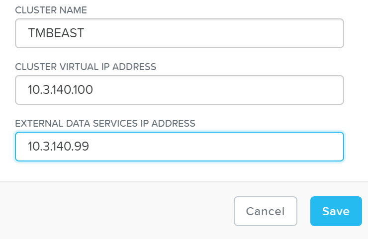
This can also be set via NCLI / API:
ncli cluster edit-params external-data- services-ip-address=<DATA SERVICES IP ADDRESS>
Target Creation
To use Block Services, the first thing we'll do is create a 'Volume Group' which is the iSCSI target.
From the 'Storage' page click on '+ Volume Group' on the right hand corner:
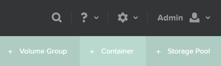
This will launch a menu where we'll specify the VG details:
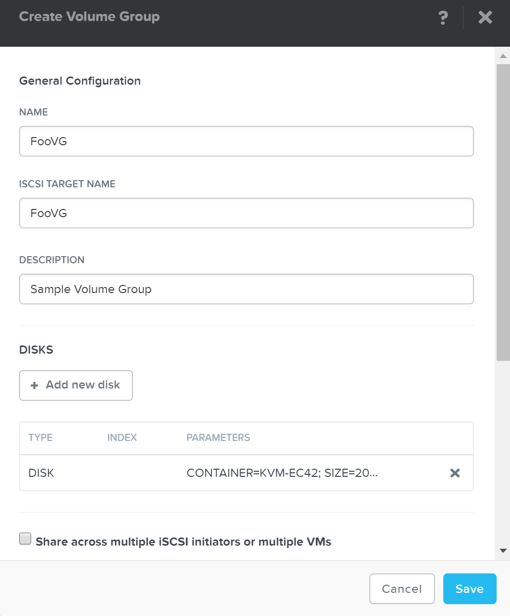
Next we'll click on '+ Add new disk' to add any disk(s) to the target (visible as LUNs):
A menu will appear allowing us to select the target container and size of the disk:
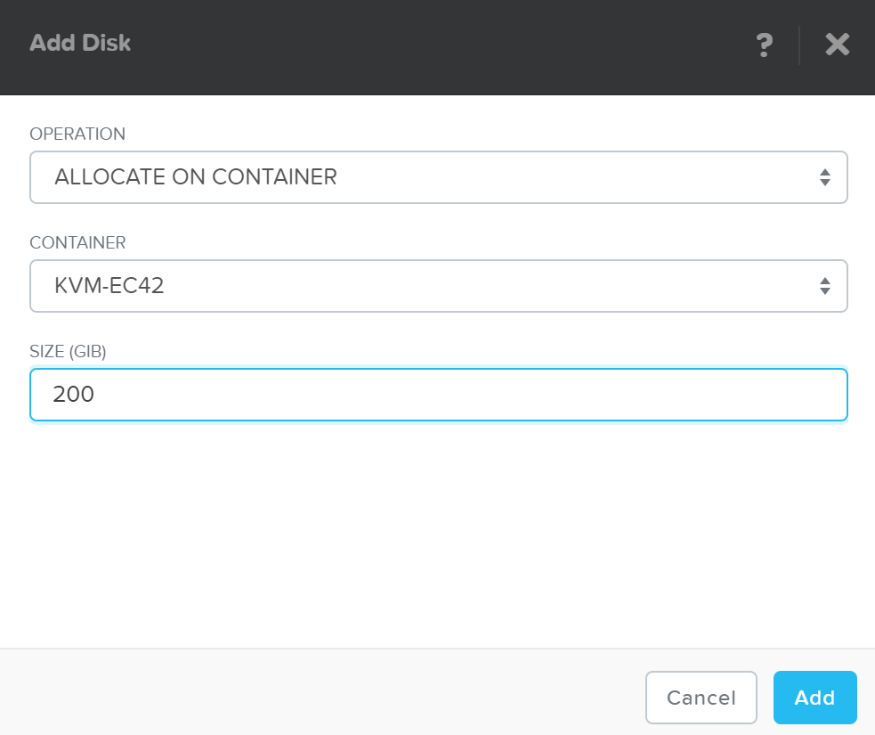
Click 'Add' and repeat this for however many disks you'd like to add.
Once we've specified the details and added disk(s) we'll attach the Volume Group to a VM or Initiator IQN. This will allow the VM to access the iSCSI target (requests from an unknown initiator are rejected):
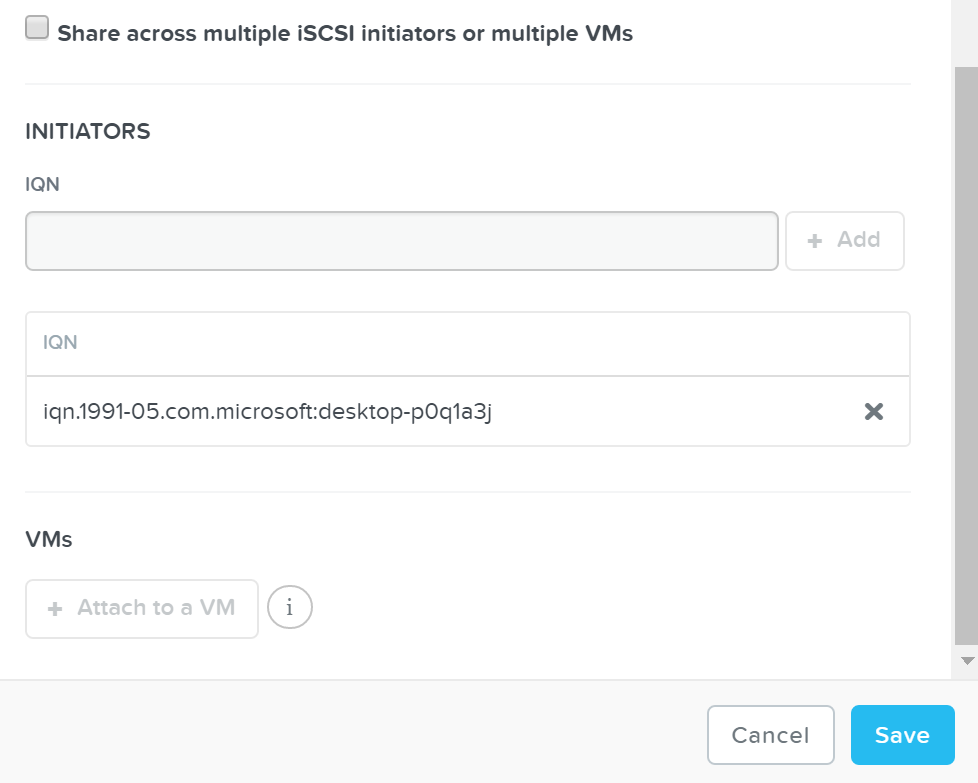
Click 'Save' and the Volume Group configuration is complete!
This can all be done via ACLI / API as well:
# Create VG
vg.create <VG Name>
# Add disk(s) to VG
Vg.disk_create <VG Name> container=<CTR Name> create_size=<Disk size, e.g. 500G>
# Attach initiator IQN to VG
Vg.attach_external <VG Name> <Initiator IQN>
Path High-Availability (HA)
As mentioned previously, the Data Services IP is leveraged for discovery. This allows for a single address that can be leveraged without the need of knowing individual CVM IP addresses.
The Data Services IP will be assigned to the current iSCSI master. In the event that fails, a new iSCSI master will become elected and assigned the Data Services IP. This ensures the discovery portal will always remain available.
The iSCSI initiator is configured with the Data Services IP as the iSCSI target portal. Upon a login request, the platform will perform an iSCSI login redirect to a healthy Stargate.
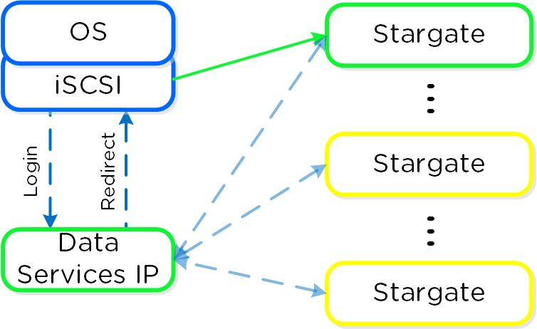
In the event where the active (affined) Stargate goes down, the initiator retries the iSCSI login to the Data Services IP, which will then redirect to another healthy Stargate.
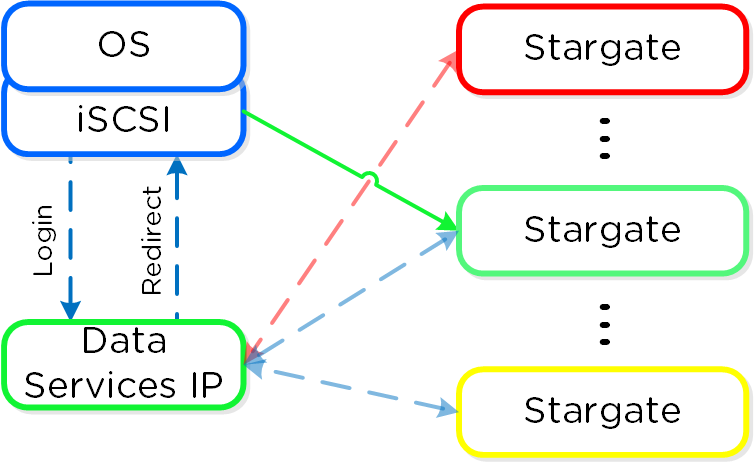
If the affined Stargate comes back up and is stable, the currently active Stargate will quiesce I/O and kill the active iSCSI session(s). When the initiator re-attempts the iSCSI login, the Data Services IP will redirect it to the affined Stargate.
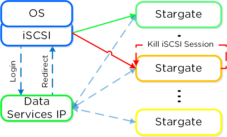
Note
Health Monitoring and Defaults
Stargate health is monitored using Zookeeper for Block Services, using the exact same mechanism as DSF.
For failback, the default interval is 120 seconds. This means once the affined Stargate is healthy for 2 or more minutes, we will quiesce and close the session. Forcing another login back to the affined Stargate.
Given this mechanism, client side multipathing (MPIO) is no longer necessary for path HA. When connecting to a target, there's now no need to check 'Enable multi-path' (which enables MPIO):
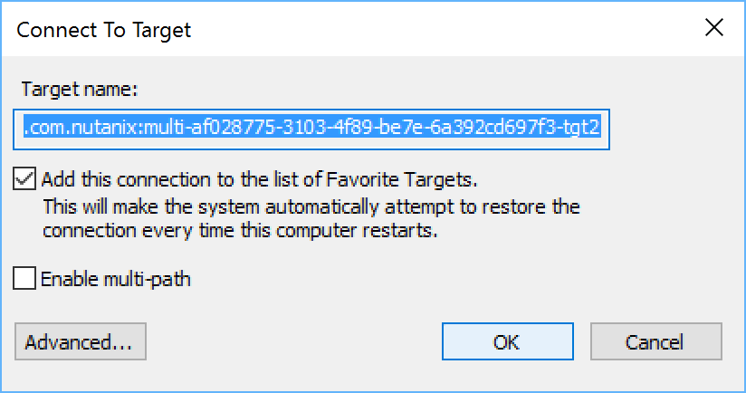
Multi-Pathing
The iSCSI protocol spec mandates a single iSCSI session (TCP connection) per target, between initiator and target. This means there a 1:1 relationship between a Stargate and a target.
As of 4.7, 32 (default) virtual targets will be automatically created per attached initiator and assigned to each disk device added to the volume group (VG). This provides an iSCSI target per disk device. Previously this would have been handled by creating multiple VGs with a single disk each.
When looking at the VG details in ACLI/API you can see the 32 virtual targets created for each attachment:
  attachment_list {
      external_initiator_name: "iqn.1991-05.com.microsoft:desktop-foo"
      target_params {
        num_virtual_targets: 32
      }
    }
Here we've created a sample VG with 3 disks devices added to it. When performing a discovery on my client I can see an individual target for each disk device (with a suffix in the format of '-tgt[int]'):
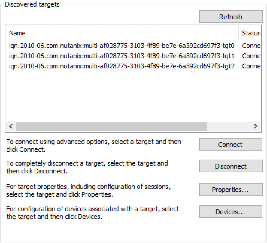
This allows each disk device to have its own iSCSI session and the ability for these sessions to be hosted across multiple Stargates, increasing scalability and performance:
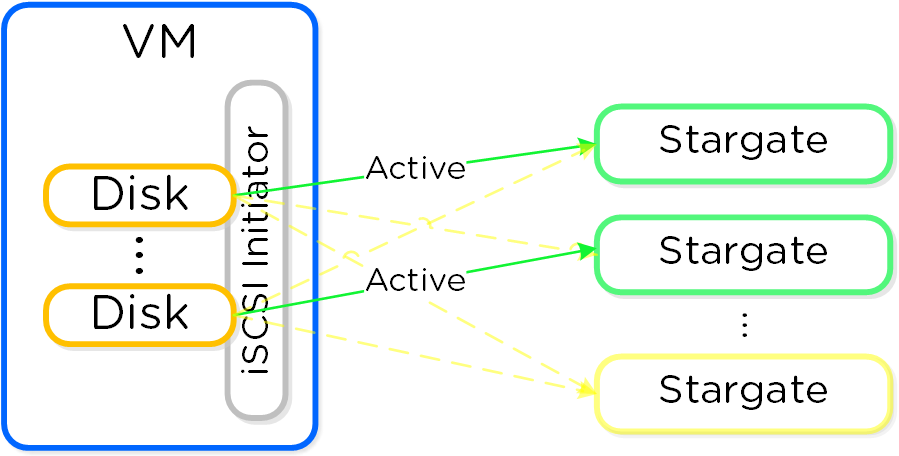
Load balancing occurs during iSCSI session establishment (iSCSI login), for each target.
As of 4.7 a simple hash function is use to distribute targets across cluster nodes. We will continue to look at the algorithm and optimize as necessary. It is also possible to set a preferred node which will be used as long as it is in a healthy state.
Note
SCSI UNMAP (TRIM)
Acropolis Block Services supports the SCSI UNMAP (TRIM) command in the SCSI T10 specification. This command is used to reclaim space from deleted blocks.
File Services
The File Services feature allows users to leverage the Nutanix platform as a highly available file server. This allows for a single namespace where users can store home directories and files.
Supported Configurations
The solution is applicable to the configurations below (list may be incomplete, refer to documentation for a fully supported list):
-
Hypervisor(s):
- AHV
- ESXi (Asterix and beyond)
-
File Protocols:
- CIFS 2.1
-
Compatible Features:
- Async-DR
File Services Constructs
This feature is composed of a few high-level constructs:
-
File Server
- High-level namespace. Each file server will have its own set of File Services VMs (FSVM) which are deployed
-
Share
- Share exposed to users. A file server can have multiple shares (e.g. departmental shares, etc.)
-
Folder
- Folders for file storage. Folders are sharded across FSVMs
The figure shows the high-level mapping of the constructs:
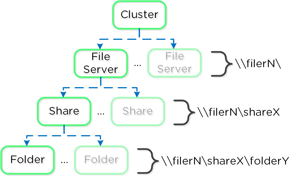
The file services feature follows the same methodology for distribution as the Nutanix platform to ensure availability and scale. A minimum of 3 FSVMs will be deployed as part of the File Server deployment.
The figure shows a detailed view of the components:
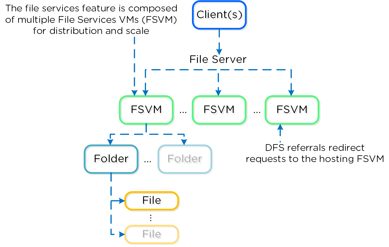
Note
Supported Protocols
As of 4.6, SMB (up to version 2.1) is the only supported protocol for client communication with file services.
The File Services VMs run as agent VMs on the platform and are transparently deployed as part of the configuration process.
The figure shows a detailed view of FSVMs on the Acropolis platform:
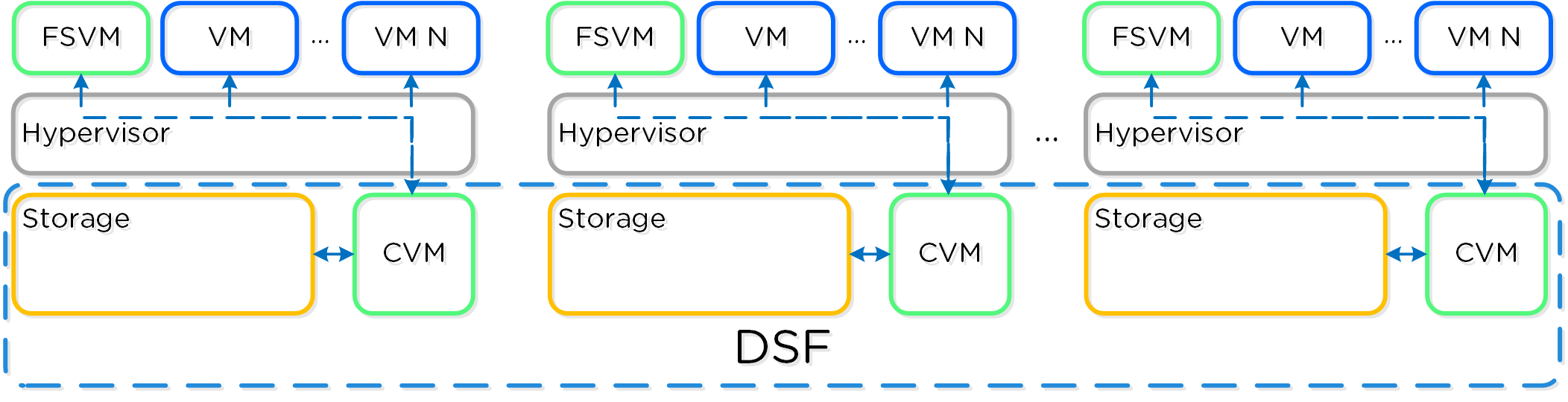
Authentication and Authorization
The File Services feature is fully integrated into Microsoft Active Directory (AD) and DNS. This allows all of the secure and established authentication and authorization capabilities of AD to be leveraged. All share permissions, user and group management is done using the traditional Windows MMC for file management.
As part of the installation process the following AD / DNS objects will be created:
- AD Computer Account for File Server
- AD Service Principal Name (SPN) for File Server and each FSVM
- DNS entry for File Server pointing to all FSVM(s)
- DNS entry for each FSVM
Note
AD Privileges for File Server Creation
A user account with the domain admin or equivalent privileges must be used to deploy the File Service feature as AD and DNS objects are created.
High-Availability (HA)
Each FSVM leverages the Acropolis Volumes API for its data storage which is accessed via in-guest iSCSI. This allows any FSVM to connect to any iSCSI target in the event of a FSVM outage.
The figure shows a high-level overview of the FSVM storage:
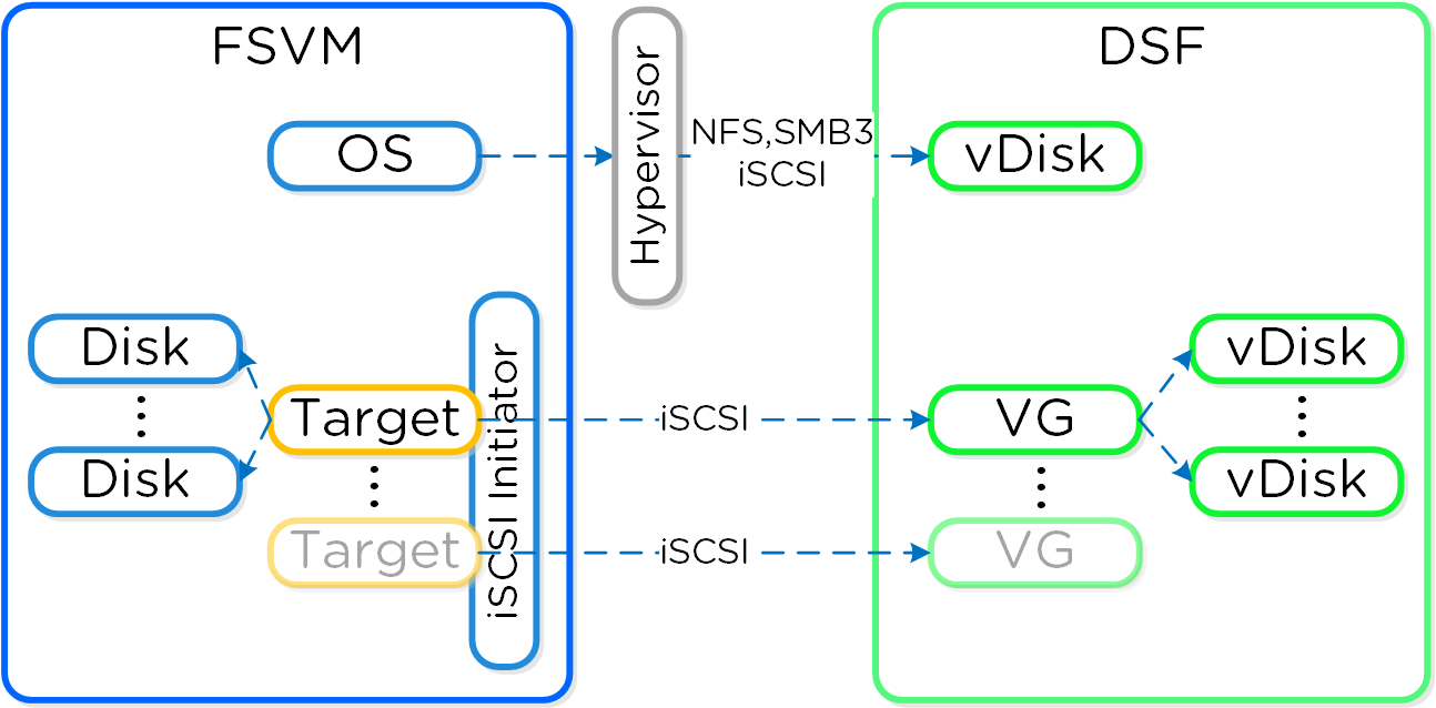
To provide for path availability DM-MPIO is leveraged within the FSVM which will have the active path set to the local CVM by default:
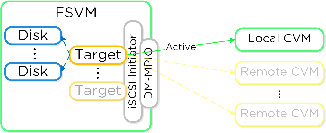
In the event where the local CVM becomes unavailable (e.g. active path down), DM-MPIO will activate one of the failover paths to a remote CVM which will then takeover IO.
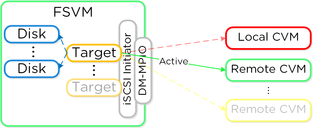
When the local CVM comes back and is healthy it will be marked as the active path to provide for local IO.
In a normal operating environment each FSVM will be communicating with its own VG for data storage with passive connections to the others. Each FSVM will have an IP which clients use to communicate with the FSVM as part of the DFS referral process. Clients do not need to know each individual FSVM's IP as the DFS referral process will connect them to the correct IP hosting their folder(s).
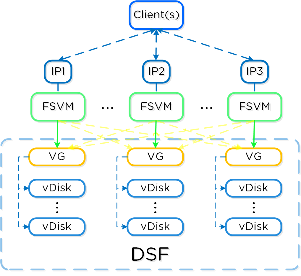
In the event of a FSVM "failure" (e.g. maintenance, power off, etc.) the VG and IP of the failed FSVM will be taken over by another FSVM to ensure client availability.
The figure shows the transfer of the failed FSVM's IP and VG:
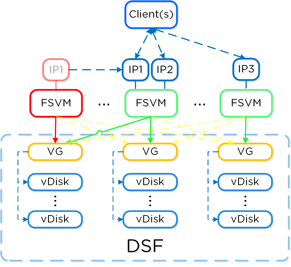
When the failed FSVM comes back and is stable, it will re-take its IP and VG and continue to serve client IO.
Container Services
Nutanix provides the ability to leverage persistent containers on the Nutanix platform using Docker (currently). It was previously possible to run Docker on Nutanix platform; however, data persistence was an issue given the ephemeral nature of containers.
Container technologies like Docker are a different approach to hardware virtualization. With traditional virtualization each VM has its own Operating System (OS) but they share the underlying hardware. Containers, which include the application and all its dependencies, run as isolated processes that share the underlying Operating System (OS) kernel.
The following table shows a simple comparison between VMs and Containers:
| Metric | Virtual Machines (VM) | Containers |
|---|---|---|
| Virtualization Type | Hardware-level virtualization | OS kernel virtualization |
| Overhead | Heavyweight | Lightweight |
| Provisioning Speed | Slower (seconds to minutes) | Real-time / fast (us to ms) |
| Performance Overhead | Limited performance | Native performance |
| Security | Fully isolated (more secure) | Process-level isolation (less secure) |
Supported Configurations
The solution is applicable to the configurations below (list may be incomplete, refer to documentation for a fully supported list):
-
Hypervisor(s):
- AHV
-
Container System(s)*:
- Docker 1.11
*As of 4.7, the solution only supports storage integration with Docker based containers. However, any other container system can run as a VM on the Nutanix platform.
Container Services Constructs
The following entities compose Acropolis Container Services:
- Nutanix Docker Host Image: Preconfigured and tested Docker host image provided by Nutanix and made available via the Nutanix Support Portal. This image is used by the Docker Machine driver for Docker host provisioning
- Nutanix Docker Machine Driver: Handles Docker container host provisioning via Docker Machine and the Acropolis Image Service
- Nutanix Docker Volume Driver: Responsible for interfacing with Acropolis Block Services to create, mount, format and attach volumes to the desired container
The following entities compose Docker (note: not all are required):
- Docker Image: The basis and image for a container
- Docker Registry: Holding space for Docker Images
- Docker Hub: Online container marketplace (public Docker Registry)
- Docker File: Text file describing how to construct the Docker image
- Docker Container: Running instantiation of a Docker Image
- Docker Engine: Creates, ships and runs Docker containers
- Docker Swarm: Docker host clustering / scheduling platform
- Docker Daemon: Handles requests from Docker Client and does heavy lifting of building, running and distributing containers
Architecture
The Nutanix solution currently leverages Docker Engine running in VMs which are created using Docker Machine. These machines can run in conjunction with normal VMs on the platform.
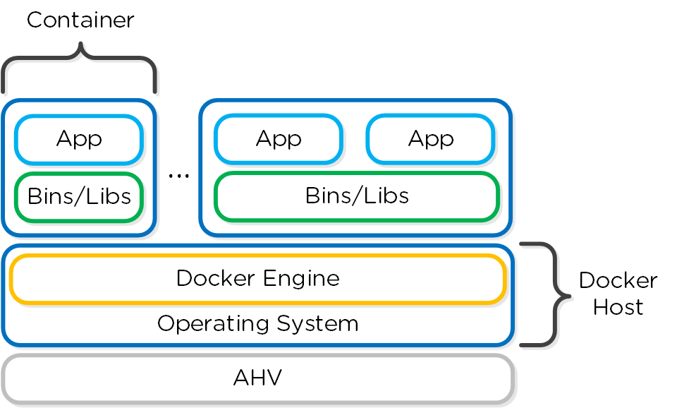
Nutanix has developed a Docker Volume Driver which will create, format and attach a volume to container(s) using the Acropolis Block Services feature. This allows the data to persist as a container is power cycled / moved.
Data persistence is achieved by using the Nutanix Volume Driver which will leverage Acropolis Block Services to attach a volume to the host / container:
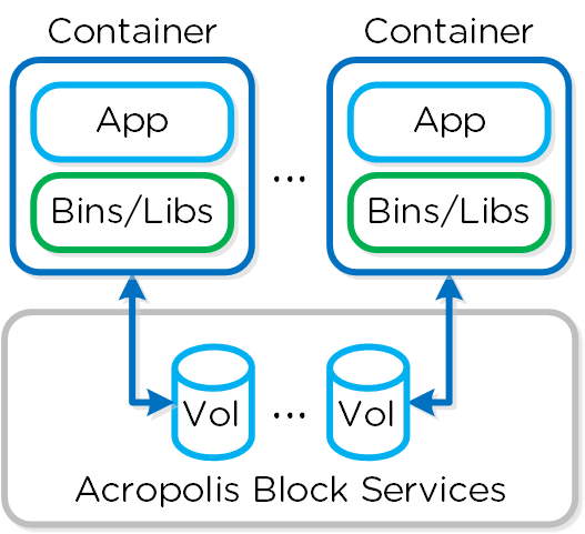
Pre-Requisites
In order for Container Services to be used the following are necessary:
- Nutanix cluster must be AOS 4.7 or later
- Nutanix Docker Host Image must be downloaded and exist as an image in the Acropolis Image Service
- The Nutanix Data Services IP must be configured
- Docker Toolbox must be installed on the client machine used for configuration
- Nutanix Docker Machine Driver must be in client's PATH
Docker Host Creation
Assuming all pre-requisites have been met the first step is to provision the Nutanix Docker Hosts using Docker Machine:
docker-machine -D create -d nutanix \ --nutanix-username <PRISM_USER> --nutanix-password <PRISM_PASSWORD> \ --nutanix-endpoint <CLUSTER_IP>:9440 --nutanix-vm-image <DOCKER_IMAGE_NAME> \ --nutanix-vm-network <NETWORK_NAME> \ --nutanix-vm-cores <NUM_CPU> --nutanix-vm-mem <MEM_MB> \ <DOCKER_HOST_NAME>
The following figure shows a high-level overview of the backend workflow:
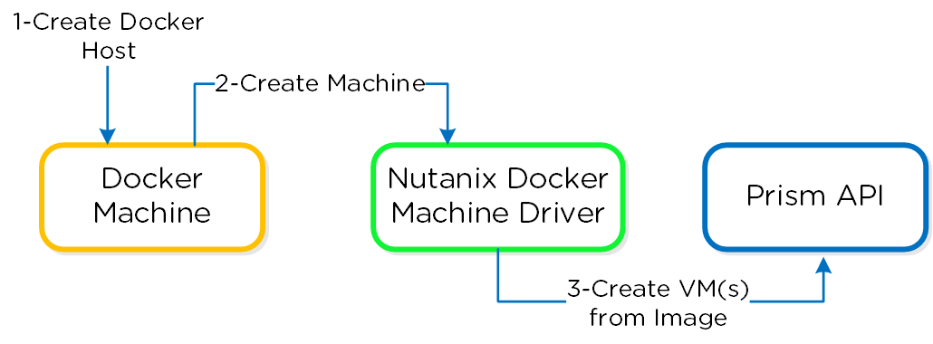
The next step is to SSH into the newly provisioned Docker Host(s) via docker-machine ssh:
docker-machine ssh <DOCKER_HOST_NAME>
Before we start the volume driver we'll make sure we have the latest driver, to pull the latest version run:
docker pull orionapps/vol-plugin
Now that we have the latest version we'll start the Nutanix Docker Volume Driver:
~/start-volume-plugin.sh
This will prompt you for the following details:
- Cluster IP
- Data Services IP
- Prism Username
- Prism Password
- Nutanix Storage Container Name
After that runs you should now see the container running the volume plugin:
[root@DOCKER-NTNX-00 ~]# docker ps
CONTAINER ID        IMAGE                  ... NAMES
37fba568078d        orionapps/vol-plugin   ... NutanixVolumePlugin
Docker Container Creation
Once the Nutanix Docker Host(s) have been deployed and the volume driver has been started, you can now provision containers with persistent storage.
These are handled using the typical Docker run command structure and specifying the Nutanix volume driver. Example usage below:
docker run -d --name <CONTAINER_NAME> \ -p <START_PORT:END_PORT> --volume-driver nutanix \ -v <VOL_NAME:VOL_MOUNT_POINT> <DOCKER_IMAGE_NAME> Example: docker run -d --name postgresexample -p 5433:5433 --volume-driver nutanix -v PGDataVol:/var/lib/postgresql/data postgres:latest
The following figure shows a high-level overview of the backend workflow:
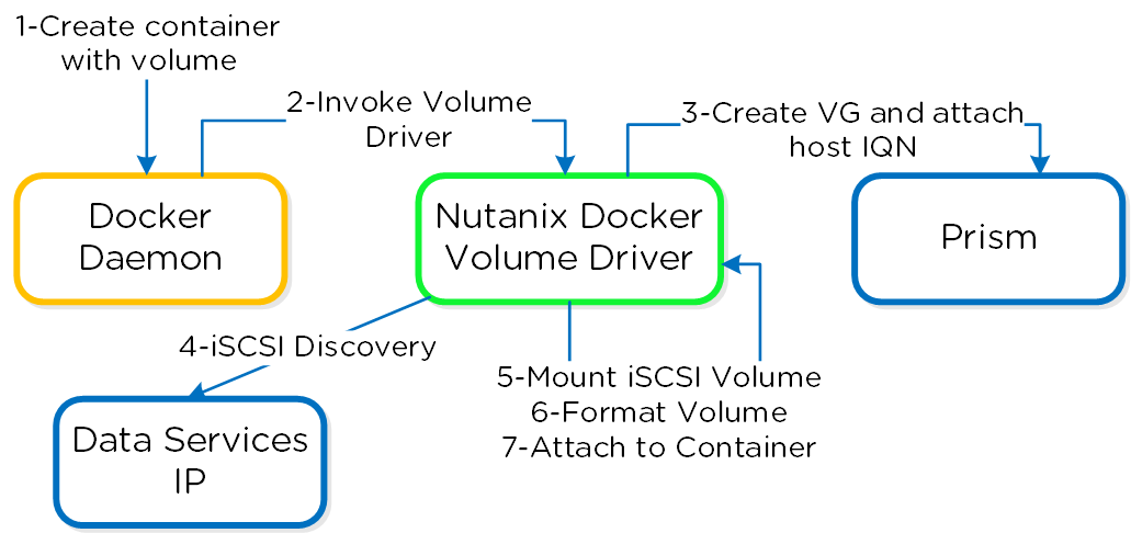
You now have a container running with persistent storage!
Backup and Disaster Recovery
Nutanix provides native backup and disaster recovery (DR) capabilities allowing users to backup, restore and DR VM(s) and objects running on DSF.
We will cover the following items in the following sections:
- Implementation Constructs
- Protecting Entities
- Backup and Restore
- Replication and DR
NOTE: Though Nutanix provides native options for backup and dr, traditional solutions (e.g. Commvault, Rubrik, etc.) can also be used, leveraging some of the native features the platform provides (VSS, snapshots, etc.).
Implementation Constructs
Within Nutanix Backup and DR, there are a few key constructs:
Protection Domain (PD)
- Key Role: Macro group of VMs and/or files to protect
- Description: A group of VMs and/or files to be replicated together on a desired schedule. A PD can protect a full container or you can select individual VMs and/or files
Note
Pro tip
Create multiple PDs for various services tiers driven by a desired RPO/RTO. For file distribution (e.g. golden images, ISOs, etc.) you can create a PD with the files to replication.
Consistency Group (CG)
- Key Role: Subset of VMs/files in PD to be crash-consistent
- Description: VMs and/or files which are part of a Protection Domain which need to be snapshotted in a crash-consistent manner. This ensures that when VMs/files are recovered, they come up in a consistent state. A protection domain can have multiple consistency groups.
Note
Pro tip
Group dependent application or service VMs in a consistency group to ensure they are recovered in a consistent state (e.g. App and DB)
Snapshot Schedule
- Key Role: Snapshot and replication schedule
- Description: Snapshot and replication schedule for VMs in a particular PD and CG
Note
Pro tip
The snapshot schedule should be equal to your desired RPO
Retention Policy
- Key Role: Number of local and remote snapshots to keep
- Description: The retention policy defines the number of local and remote snapshots to retain. NOTE: A remote site must be configured for a remote retention/replication policy to be configured.
Note
Pro tip
The retention policy should equal the number of restore points required per VM/file
Remote Site
- Key Role: A remote Nutanix cluster
- Description: A remote Nutanix cluster which can be leveraged as a target for backup or DR purposes.
Note
Pro tip
Ensure the target site has ample capacity (compute/storage) to handle a full site failure. In certain cases replication/DR between racks within a single site can also make sense.
The following figure shows a logical representation of the relationship between a PD, CG, and VM/Files for a single site:
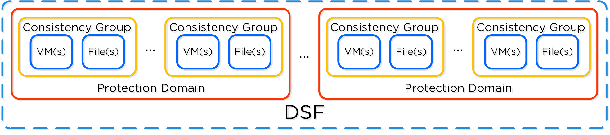
Protecting Entities
You can protect Entities (VMs, VGs, Files), using the following workflow:
From the Data Protection page, select + Protection Domain -> Async DR:
Specify a PD name and click 'Create'
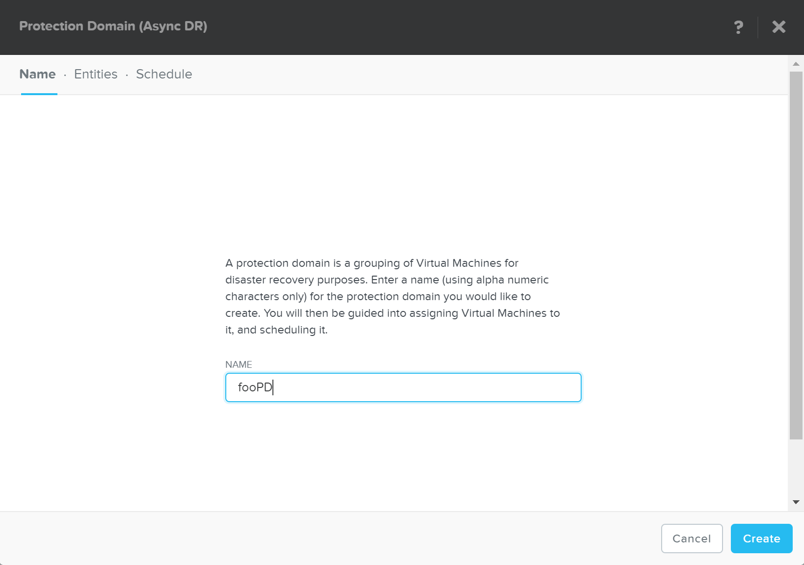
Select entities to protect:
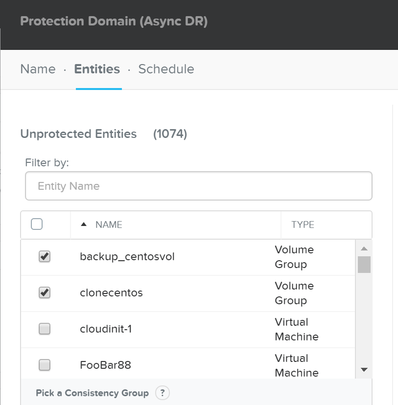
Click 'Protect Selected Entities'
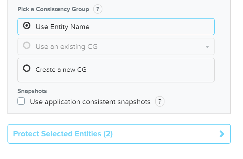
The protect entities will now be displayed under 'Protected Entities'
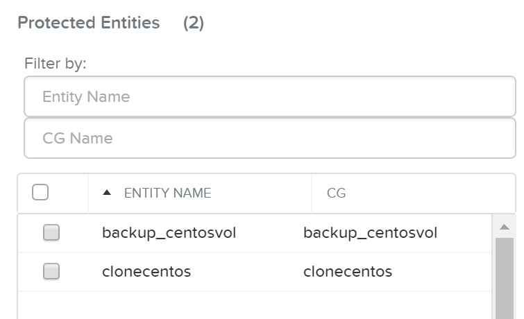
Click 'Next', then click 'Next Schedule' to create a snapshot and replication schedule
Enter the desired snapshot frequency, retention and any remote sites for replication
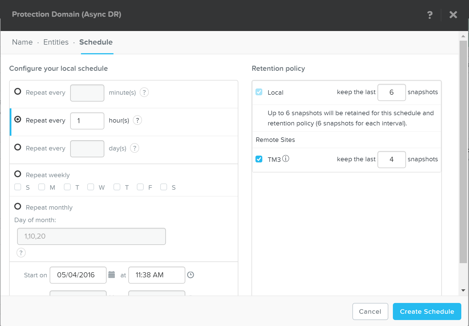
Click 'Create Schedule' to complete the schedule completion.
Note
Multiple Schedules
It is possible to create multiple snapshot / replication schedules. For example, if you want to have a local backup schedule occurring hourly and another schedule which replicated to a remote site daily.
It’s important to mention that a full container can be protected for simplicity. However, the platform provides the ability to protect down to the granularity of a single VM and/or file level.
Backup and Restore
Nutanix backup capabilities leverage the native DSF snapshot capabilities and are invoked by Cerebro and performed by Stargate. These snapshot capabilities are zero copy to ensure efficient storage utilization and low overhead. You can read more on Nutanix snapshots in the 'Snapshots and Clones' section.
Typical backup and restore operations include:
- Snapshot: Create a restore point and replicate (if necessary)
- Restore: Restore VM(s) / File(s) from a previous snapshot (replaces original objects)
- Clone: Similar to restore but does not replace original objects (creates new objects as desired snapshot)
From the Data Protection Page, you can see the protection domains (PD) previously created in the 'Protecting Entities' section.
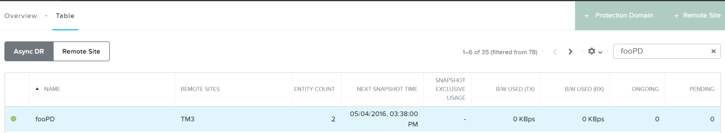
Once you're selected a target PD you can see the various options:

If you click 'Take Snapshot' you can take an ad-hoc snapshot of the selected PD and replicate to a remote site if necessary:
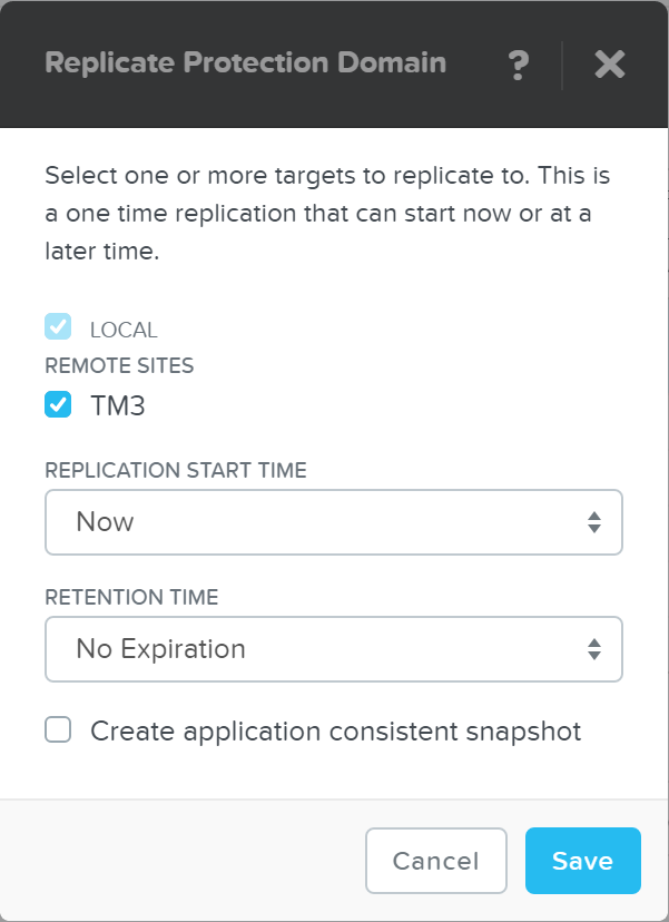
You can also 'Migrate' the PD which will fail over the entities to a remote site:
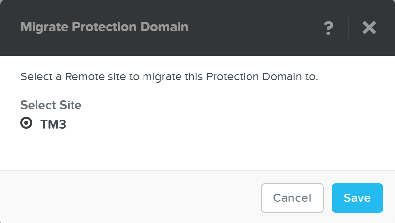
In the event of a migrate (controlled failover), the system will take a new snapshot, replicate then promote the other site with the newly created snap.
Note
Pro tip
With Asterix and above you can now leverage a single node replication target data protection.
You can also view the PD snapshot(s) in the table below:
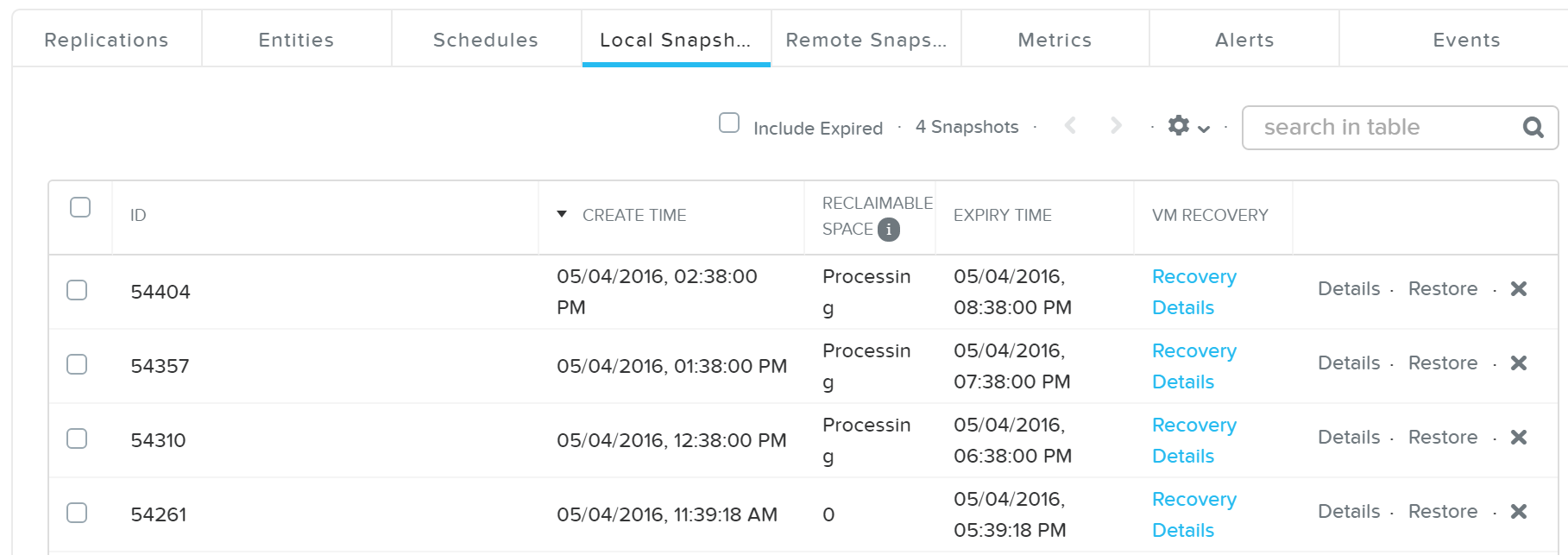
From here you can restore or clone a PD snapshot:
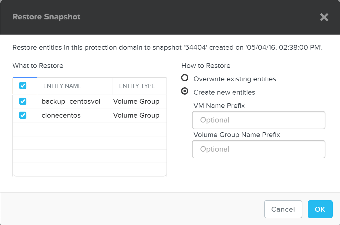
If you choose to 'Create new entities' that will be like cloning the snapshot of the PD to new entities with the desired prefixes. Otherwise 'Overwrite existing entities' will replace the current entities with those at the time of the snapshot.
Note
Storage only backup target
For backup / archival only purposes, it is possible to configure a storage only Nutanix cluster as a remote site which will act as a backup target. This will allow data to be replicated to / from the storage only cluster.
App Consistent Snapshots
Nutanix provides native VmQueisced Snapshot Service (VSS) capabilities for queiscing OS and application operations which ensure an application consistent snapshot is achieved.
Note
VmQueisced Snapshot Service (VSS)
VSS is typically a Windows specific term for Volume Shadow Copy Service. However, since this solution applies to both Windows and Linux we've modified the term to VmQueisced Snapshot Service.
Supported Configurations
The solution is applicable to both Windows and Linux guests, including versions below (list may be incomplete, refer to documentation for a fully supported list):
-
Hypervisors:
- ESX
- AHV
-
Windows
- 2008R2, 2012, 2012R2
-
Linux
- CentOS 6.5/7.0
- RHEL 6.5/7.0
- OEL 6.5/7.0
- Ubuntu 14.04+
- SLES11SP3+
Pre-Requisites
In order for Nutanix VSS snapshots to be used the following are necessary:
-
Nutanix Platform
- Cluster Virtual IP (VIP) must be configured
-
Guest OS / UVM
- NGT must be installed
- CVM VIP must be reachable on port 2074
-
Disaster Recovery Configuration
- UVM must be in PD with 'Use application consistent snapshots' enabled
Architecture
As of 4.6 this is achieved using the native Nutanix Hardware VSS provider which is installed as part of the Nutanix Guest Tools package. You can read more on the guest tools in the 'Nutanix Guest Tools' section.
The following image shows a high-level view of the VSS architecture:
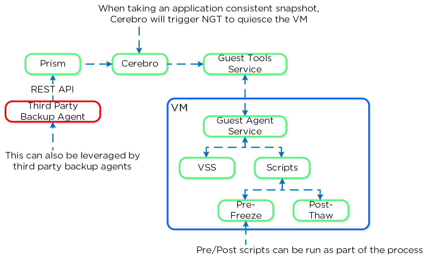
You can perform an application consistent snapshot by following the normal data protection workflow and selecting 'Use application consistent snapshots' when protecting the VM.
Note
Enabling/Disabling Nutanix VSS
When NGT is enabled for a UVM, the Nutanix VSS snapshot capability is enabled by default. However, you can turn off this capability with the following command:
ncli ngt disable-applications application-names=vss_snapshot vm_id=<VM_ID>
Windows VSS Architecture
The Nutanix VSS solution is integrated with the Windows VSS framework. The following shows a high-level view of the architecture:
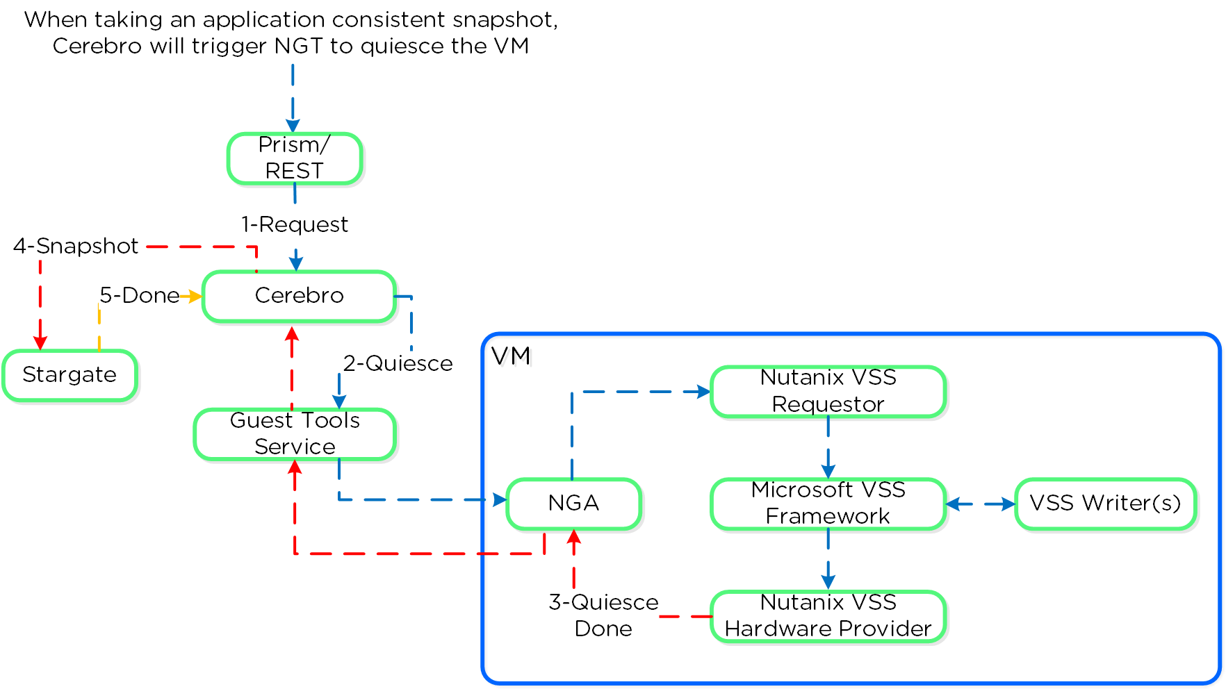
Once NGT is installed you can see the NGT Agent and VSS Hardware Provider services:
Linux VSS Architecture
The Linux solution works similar to the Windows solution, however scripts are leveraged instead of the Microsoft VSS framework as it doesn't exist in Linux distros.
The Nutanix VSS solution is integrated with the Windows VSS framework. The following shows a high-level view of the architecture:
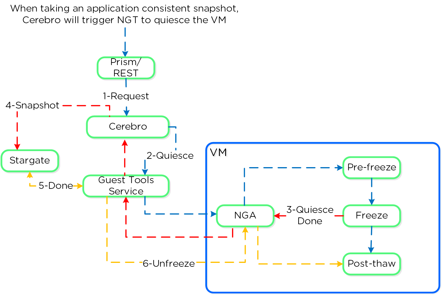
The pre-freeze and post-thaw scripts are located in the following directories:
- Pre-freeze: /sbin/pre_freeze
- Post-thaw: /sbin/post-thaw
Note
Eliminating ESXi Stun
ESXi has native app consistent snapshot support using VMware guest tools. However, during this process, delta disks are created and ESXi "stuns" the VM in order to remap the virtual disks to the new delta files which will handle the new write IO. Stuns will also occur when a VMware snapshot is deleted.
During this stun process the VM its OS cannot execute any operations and is essentially in a "stuck" state (e.g. pings will fail, no IO). The duration of the stun will depend on the number of vmdks and speed of datastore metadata operations (e.g. create new delta disks, etc.)
By using Nutanix VSS we completely bypass the VMware snapshot / stun process and have little to no impact to performance or VM / OS availability.
Replication and Disaster Recovery (DR)
For a visual explanation, you can watch the following video: LINK
Nutanix provides native DR and replication capabilities, which build upon the same features explained in the Snapshots & Clones section. Cerebro is the component responsible for managing the DR and replication in DSF. Cerebro runs on every node and a Cerebro master is elected (similar to NFS master) and is responsible for managing replication tasks. In the event the CVM acting as Cerebro master fails, another is elected and assumes the role. The Cerebro page can be found on <CVM IP>:2020. The DR function can be broken down into a few key focus areas:
- Replication Topologies
- Replication Lifecycle
- Global Deduplication
Replication Topologies
Traditionally, there are a few key replication topologies: Site to site, hub and spoke, and full and/or partial mesh. Contrary to traditional solutions which only allow for site to site or hub and spoke, Nutanix provides a fully mesh or flexible many-to-many model.
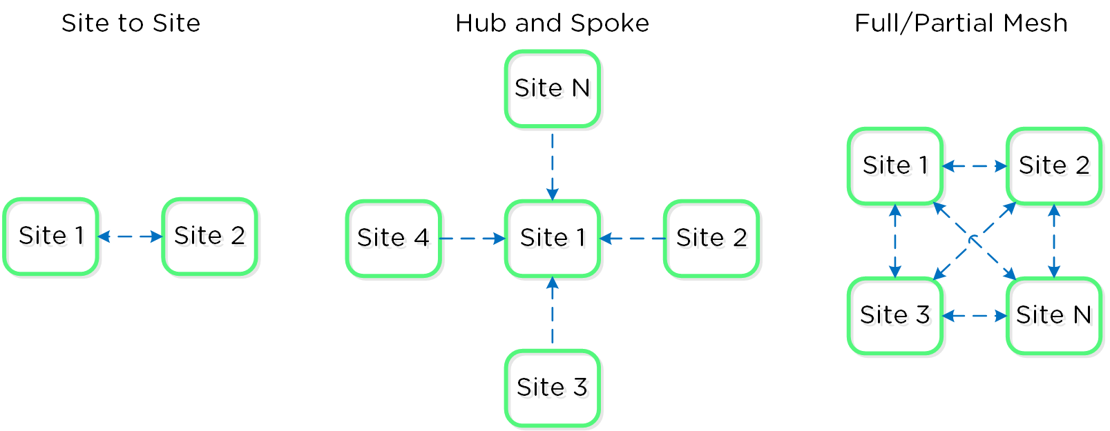
Essentially, this allows the admin to determine a replication capability that meets their company's needs.
Replication Lifecycle
Nutanix replication leverages the Cerebro service mentioned above. The Cerebro service is broken into a “Cerebro Master”, which is a dynamically elected CVM, and Cerebro Slaves, which run on every CVM. In the event where the CVM acting as the “Cerebro Master” fails, a new “Master” is elected.
The Cerebro Master is responsible for managing task delegation to the local Cerebro Slaves as well as coordinating with remote Cerebro Master(s) when remote replication is occurring.
During a replication, the Cerebro Master will figure out which data needs to be replicated, and delegate the replication tasks to the Cerebro Slaves which will then tell Stargate which data to replicate and to where.
Replicated data is protected at multiple layers throughout the process. Extent reads on the source are checksummed to ensure consistency for source data (similar to how any DSF read occurs) and the new extent(s) are checksummed at the target (similar to any DSF write). TCP provides consistency on the network layer.
The following figure shows a representation of this architecture:
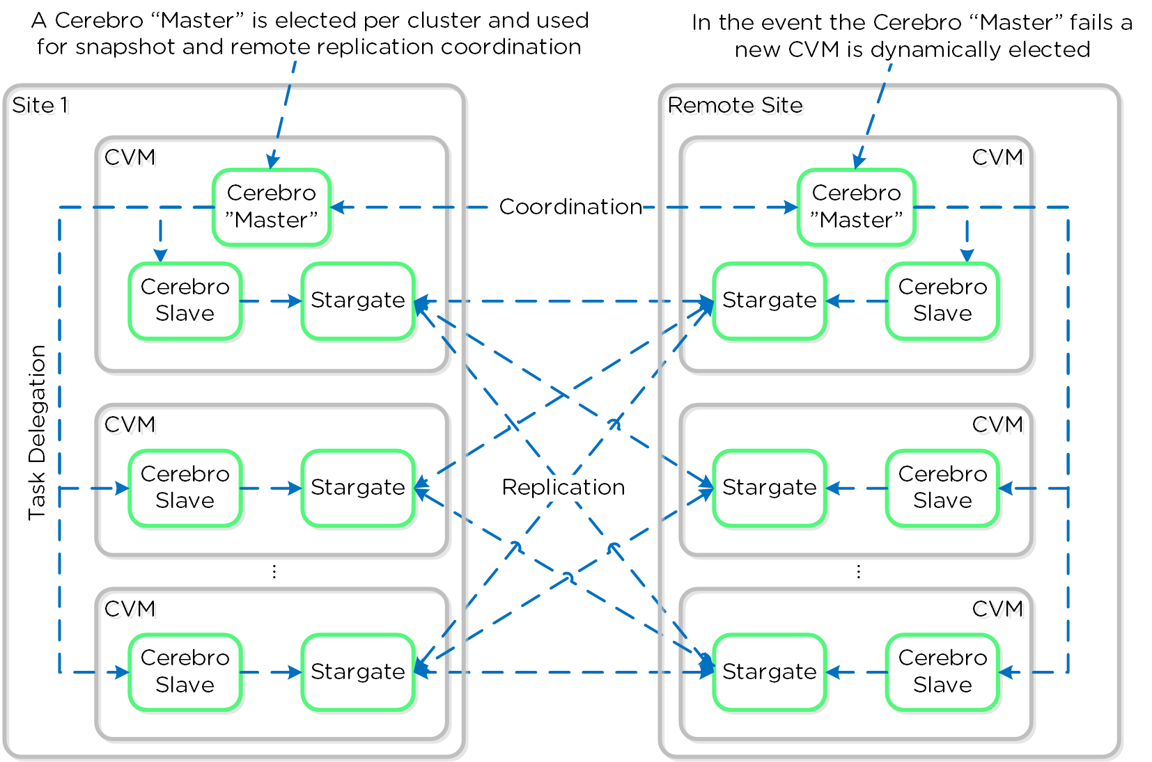
It is also possible to configure a remote site with a proxy which will be used as a bridgehead for all coordination and replication traffic coming from a cluster.
Note
Pro tip
When using a remote site configured with a proxy, always utilize the cluster IP as that will always be hosted by the Prism Leader and available, even if CVM(s) go down.
The following figure shows a representation of the replication architecture using a proxy:
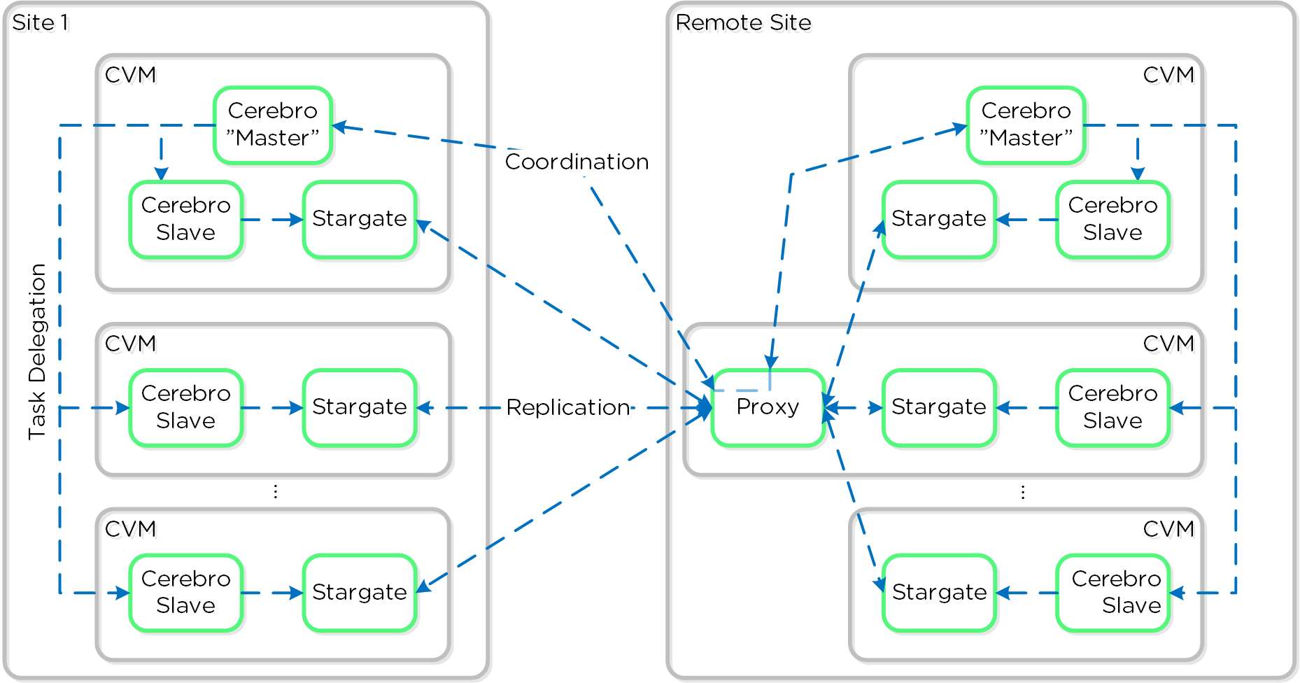
In certain scenarios, it is also possible to configure a remote site using a SSH tunnel where all traffic will flow between two CVMs.
Note
Note
This should only be used for non-production scenarios and the cluster IPs should be used to ensure availability.The following figure shows a representation of the replication architecture using a SSH tunnel:
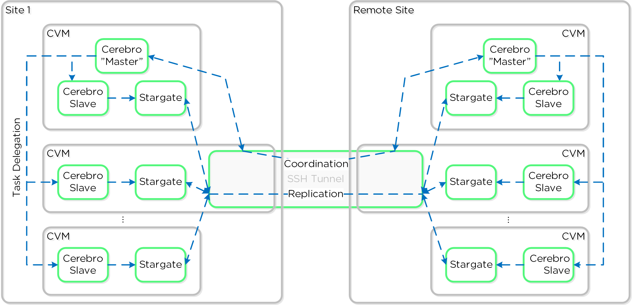
Global Deduplication
As explained in the Elastic Deduplication Engine section above, DSF has the ability to deduplicate data by just updating metadata pointers. The same concept is applied to the DR and replication feature. Before sending data over the wire, DSF will query the remote site and check whether or not the fingerprint(s) already exist on the target (meaning the data already exists). If so, no data will be shipped over the wire and only a metadata update will occur. For data which doesn’t exist on the target, the data will be compressed and sent to the target site. At this point, the data exists on both sites is usable for deduplication.
The following figure shows an example three site deployment where each site contains one of more protection domains (PD):
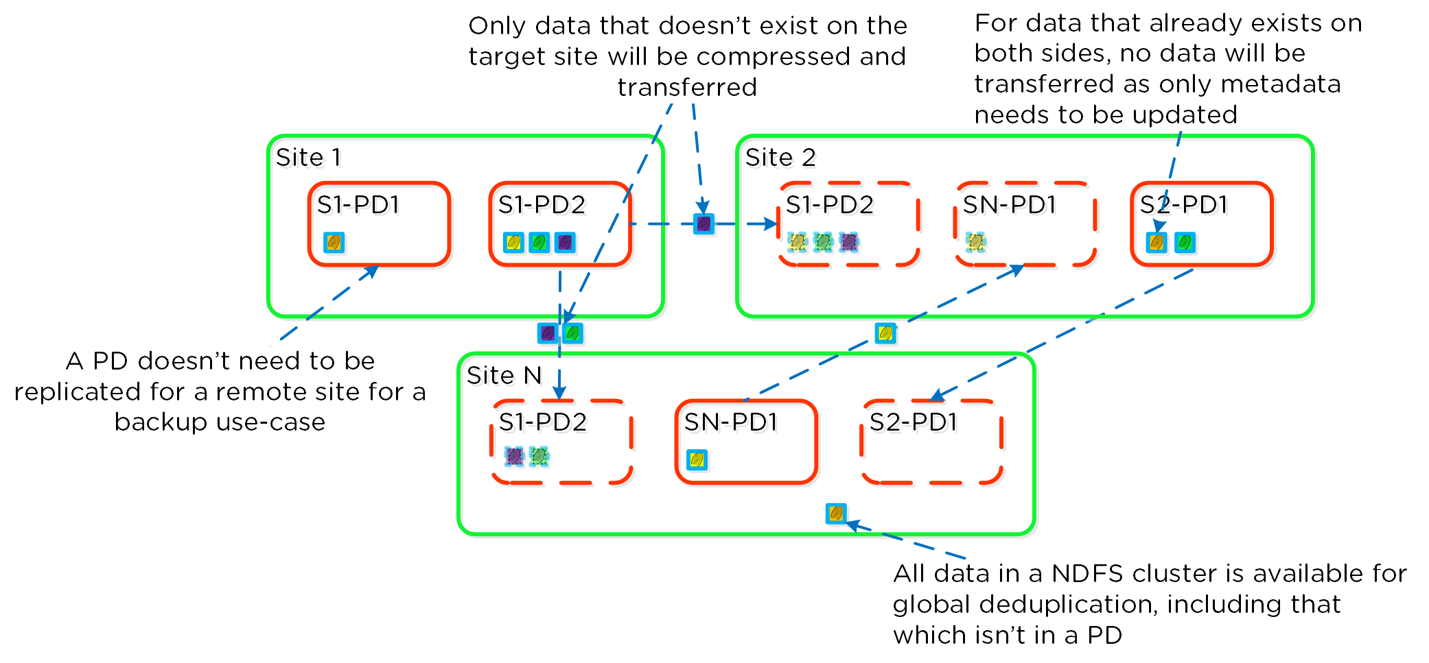
Note
Note
Fingerprinting must be enabled on the source and target container / vstore for replication deduplication to occur.
Cloud Connect
Building upon the native DR / replication capabilities of DSF, Cloud Connect extends this capability into cloud providers (currently Amazon Web Services, Microsoft Azure). NOTE: This feature is currently limited to just backup / replication.
Very similar to creating a remote site to be used for native DR / replication, a “cloud remote site” is just created. When a new cloud remote site is created, Nutanix will automatically spin up a single node Nutanix cluster in EC2 (currently m1.xlarge) or Azure Virtual Machines (currently D3) to be used as the endpoint.
The cloud instance is based upon the same Acropolis code-base leveraged for locally running clusters. This means that all of the native replication capabilities (e.g., global deduplication, delta based replications, etc.) can be leveraged.
In the case where multiple Nutanix clusters are leveraging Cloud Connect, they can either A) share the same instance running in the region, or B) spin up a new instance.
Storage for cloud instances is done using a "cloud disk" which is a logical disk backed by S3 (AWS) or BlobStore (Azure). Data is stored as the usual egroups which are files on the object stores.
The following figure shows a logical representation of a “remote site” used for Cloud Connect:
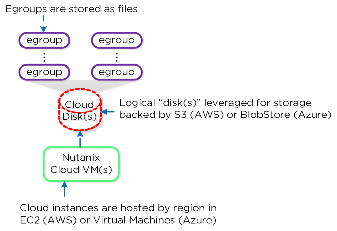
Since a cloud based remote site is similar to any other Nutanix remote site, a cluster can replicate to multiple regions if higher availability is required (e.g., data availability in the case of a full region outage):
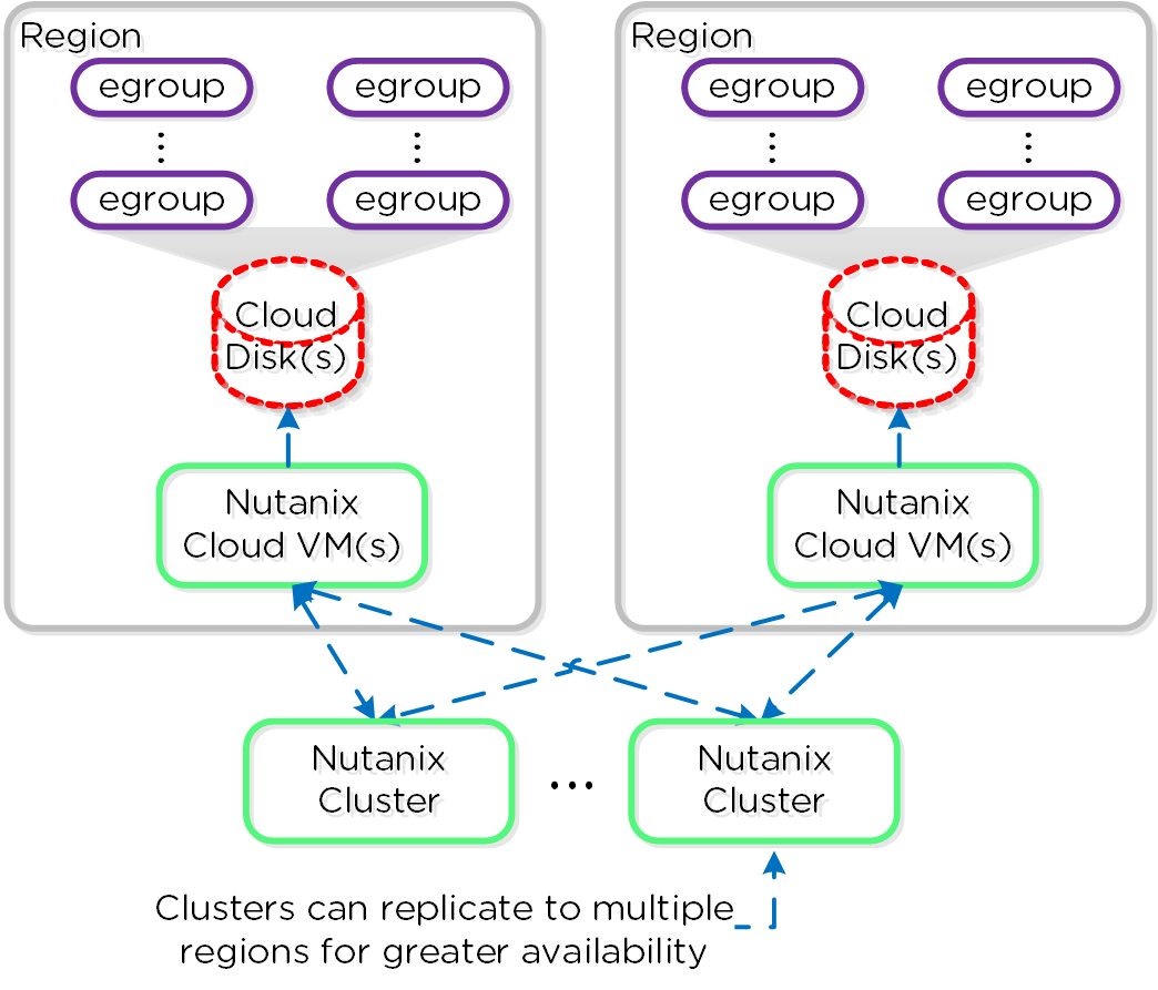
The same replication / retention policies are leveraged for data replicated using Cloud Connect. As data / snapshots become stale, or expire, the cloud cluster will clean up data as necessary.
If replication isn’t frequently occurring (e.g., daily or weekly), the platform can be configured to power up the cloud instance(s) prior to a scheduled replication and down after a replication has completed.
Data that is replicated to any cloud region can also be pulled down and restored to any existing, or newly created Nutanix cluster which has the cloud remote site(s) configured:
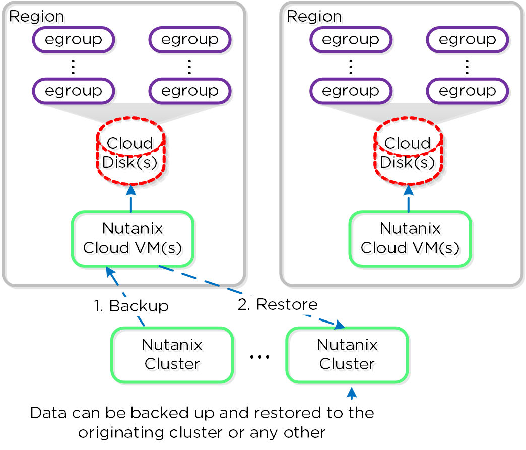
Metro Availability
Nutanix provides native “stretch clustering” capabilities which allow for a compute and storage cluster to span multiple physical sites. In these deployments, the compute cluster spans two locations and has access to a shared pool of storage.
This expands the VM HA domain from a single site to between two sites providing a near 0 RTO and a RPO of 0.
In this deployment, each site has its own Nutanix cluster, however the containers are “stretched” by synchronously replicating to the remote site before acknowledging writes.
The following figure shows a high-level design of what this architecture looks like:
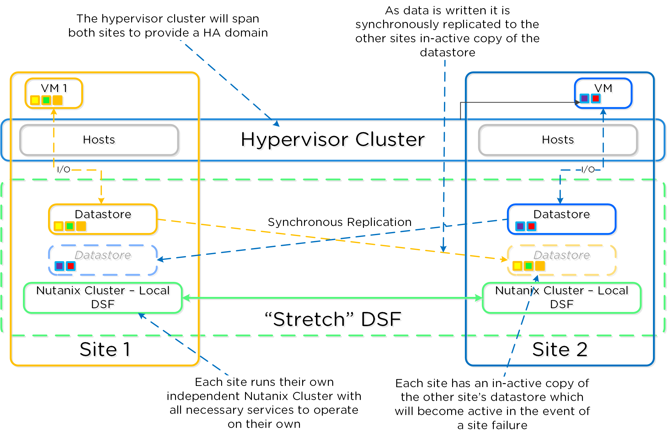
In the event of a site failure, an HA event will occur where the VMs can be restarted on the other site. The failover process is typically a manual process. With the Asterix release a Metro Witness can be configured which can automate the failover. The witness can be downloaded via the Portal and is configured via Prism.
The following figure shows an example site failure:
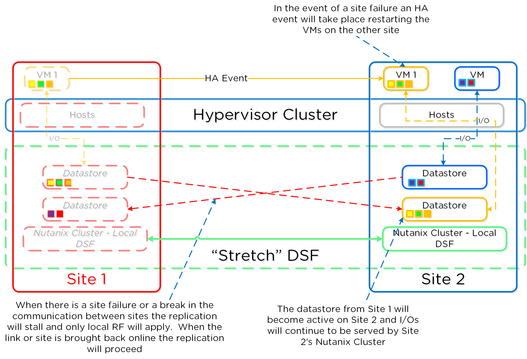
In the event where there is a link failure between the two sites, each cluster will operate independently. Once the link comes back up, the sites will be re-synchronized (deltas-only) and synchronous replication will start occurring.
The following figure shows an example link failure:
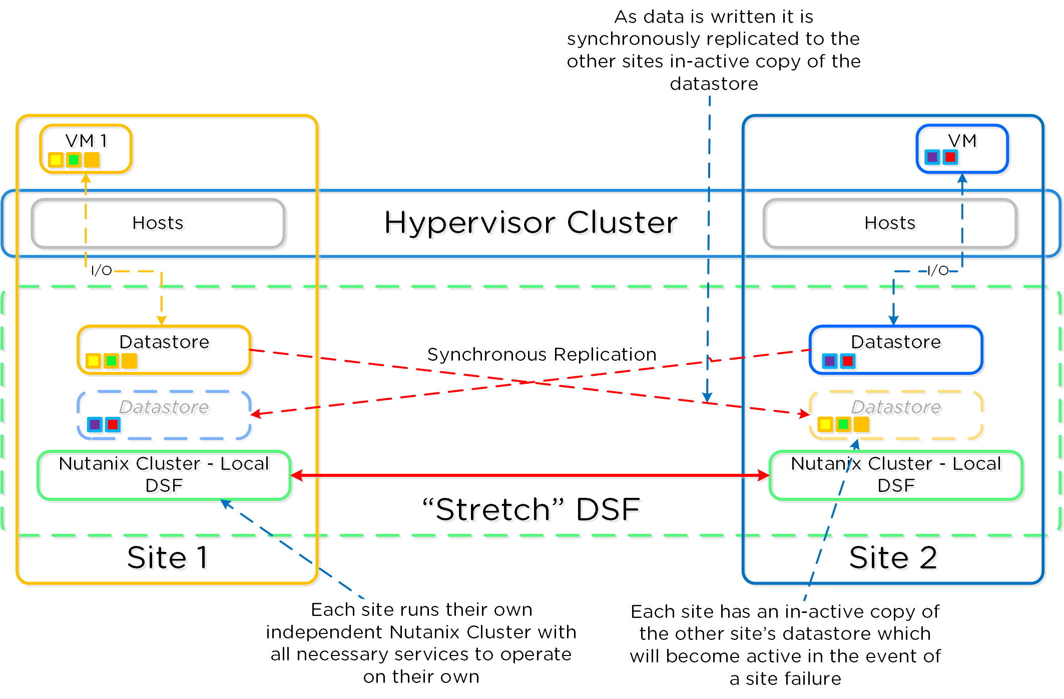
Application Mobility Fabric - coming soon!
More coming soon!
Administration
Important Pages
These are advanced Nutanix pages besides the standard user interface that allow you to monitor detailed stats and metrics. The URLs are formatted in the following way: http://<Nutanix CVM IP/DNS>:<Port/path (mentioned below)> Example: http://MyCVM-A:2009 NOTE: if you’re on a different subnet IPtables will need to be disabled on the CVM to access the pages.
2009 Page
This is a Stargate page used to monitor the back end storage system and should only be used by advanced users. I’ll have a post that explains the 2009 pages and things to look for.
2009/latency Page
This is a Stargate page used to monitor the back end latency.
2009/vdisk_stats Page
This is a Stargate page used to show various vDisk stats including histograms of I/O sizes, latency, write hits (e.g., OpLog, eStore), read hits (cache, SSD, HDD, etc.) and more.
2009/h/traces Page
This is the Stargate page used to monitor activity traces for operations.
2009/h/vars Page
This is the Stargate page used to monitor various counters.
2010 Page
This is the Curator page which is used for monitoring Curator runs.
2010/master/control Page
This is the Curator control page which is used to manually start Curator jobs
2011 Page
This is the Chronos page which monitors jobs and tasks scheduled by Curator.
2020 Page
This is the Cerebro page which monitors the protection domains, replication status and DR.
2020/h/traces Page
This is the Cerebro page used to monitor activity traces for PD operations and replication.
2030 Page
This is the main Acropolis page and shows details about the environment hosts, any currently running tasks and networking details.
2030/sched Page
This is an Acropolis page used to show information about VM and resource scheduling used for placement decisions. This page shows the available host resources and VMs running on each host.
2030/tasks Page
This is an Acropolis page used to show information about Acropolis tasks and their state. You can click on the task UUID to get detailed JSON about the task.
2030/vms Page
This is an Acropolis page used to show information about Acropolis VMs and details about them. You can click on the VM Name to connect to the console.
Cluster Commands
Check cluster status
Description: Check cluster status from the CLI
cluster status
Check local CVM service status
Description: Check a single CVM's service status from the CLI
genesis status
Nutanix cluster upgrade
Description: Perform rolling (aka "live") cluster upgrade from the CLI
Upload upgrade package to ~/tmp/ on one CVM
Untar package
tar xzvf ~/tmp/nutanix*
Perform upgrade
~/tmp/install/bin/cluster -i ~/tmp/install upgrade
Check status
upgrade_status
Node(s) upgrade
Description: Perform upgrade of specified node(s) to current clusters version
From any CVM running the desired version run the following command:
cluster -u <NODE_IP(s)> upgrade_node
Hypervisor upgrade status
Description: Check hypervisor upgrade status from the CLI on any CVM
host_upgrade --status
Detailed logs (on every CVM)
~/data/logs/host_upgrade.out
Restart cluster service from CLI
Description: Restart a single cluster service from the CLI
Stop service
cluster stop <Service Name>
Start stopped services
cluster start #NOTE: This will start all stopped services
Start cluster service from CLI
Description: Start stopped cluster services from the CLI
Start stopped services
cluster start #NOTE: This will start all stopped services
OR
Start single service
Start single service: cluster start <Service Name>
Restart local service from CLI
Description: Restart a single cluster service from the CLI
Stop Service
genesis stop <Service Name>
Start Service
cluster start
Start local service from CLI
Description: Start stopped cluster services from the CLI
cluster start #NOTE: This will start all stopped services
Cluster add node from cmdline
Description: Perform cluster add-node from CLI
ncli cluster discover-nodes | egrep "Uuid" | awk '{print $4}' | xargs -I UUID ncli cluster add-node node-uuid=UUID
Find cluster id
Description: Find the cluster ID for the current cluster
zeus_config_printer | grep cluster_id
Open port
Description: Enable port through IPtables
sudo vi /etc/sysconfig/iptables
-A INPUT -m state --state NEW -m tcp -p tcp --dport <PORT> -j ACCEPT
sudo service iptables restart
Check for Shadow Clones
Description: Displays the shadow clones in the following format: name#id@svm_id
vdisk_config_printer | grep '#'
Reset Latency Page Stats
Description: Reset the Latency Page (<CVM IP>:2009/latency) counters
allssh "wget 127.0.0.1:2009/latency/reset"
Find vDisk information
Description: Find vDisk information and details including name, id, size, iqn and others
vdisk_config_printer
Find Number of vDisks
Description: Find the current number of vDisks (files) on DSF
vdisk_config_printer | grep vdisk_id | wc -l
Get detailed vDisk information
Description: Displays a provided vDisks egroup IDs, size, transformation and savings, garbage and replica placement
vdisk_usage_printer -vdisk_id=<VDISK_ID>
Start Curator scan from CLI
Description: Starts a Curator scan from the CLI
# Full Scan
allssh "wget -O - "http://localhost:2010/master/api/client/StartCuratorTasks?task_type=2";"
# Partial Scan
allssh "wget -O - "http://localhost:2010/master/api/client/StartCuratorTasks?task_type=3";"
# Refresh Usage
allssh "wget -O - "http://localhost:2010/master/api/client/RefreshStats";"
Check under replicated data via CLI
Description: Check for under replicated data using curator_cli
curator_cli get_under_replication_info summary=true
Compact ring
Description: Compact the metadata ring
allssh "nodetool -h localhost compact"
Find NOS version
Description: Find the NOS version (NOTE: can also be done using NCLI)
allssh "cat /etc/nutanix/release_version"
Find CVM version
Description: Find the CVM image version
allssh "cat /etc/nutanix/svm-version"
Manually fingerprint vDisk(s)
Description: Create fingerprints for a particular vDisk (For dedupe) NOTE: dedupe must be enabled on the container
vdisk_manipulator –vdisk_id=<vDisk ID> --operation=add_fingerprints
Echo Factory_Config.json for all cluster nodes
Description: Echos the factory_config.jscon for all nodes in the cluster
allssh "cat /etc/nutanix/factory_config.json"
Upgrade a single Nutanix node’s NOS version
Description: Upgrade a single node's NOS version to match that of the cluster
~/cluster/bin/cluster -u <NEW_NODE_IP> upgrade_node
List files (vDisk) on DSF
Description: List files and associated information for vDisks stored on DSF
Nfs_ls
Get help text
Nfs_ls --help
Install Nutanix Cluster Check (NCC)
Description: Installs the Nutanix Cluster Check (NCC) health script to test for potential issues and cluster health
Download NCC from the Nutanix Support Portal (portal.nutanix.com)
SCP .tar.gz to the /home/nutanix directory
Untar NCC .tar.gz
tar xzmf <ncc .tar.gz file name> --recursive-unlink
Run install script
./ncc/bin/install.sh -f <ncc .tar.gz file name>
Create links
source ~/ncc/ncc_completion.bash
echo "source ~/ncc/ncc_completion.bash" >> ~/.bashrc
Run Nutanix Cluster Check (NCC)
Description: Runs the Nutanix Cluster Check (NCC) health script to test for potential issues and cluster health. This is a great first step when troubleshooting any cluster issues.
Make sure NCC is installed (steps above)
Run NCC health checks
ncc health_checks run_all
List tasks using progress monitor cli
progress_monitor_cli -fetchall
Remove task using progress monitor cli
progress_monitor_cli --entity_id=<ENTITY_ID> --operation=<OPERATION> --entity_type=<ENTITY_TYPE> --delete
# NOTE: operation and entity_type should be all lowercase with k removed from the begining
Metrics and Thresholds
The following section will cover specific metrics and thresholds on the Nutanix back end. More updates to these coming shortly!
Gflags
More coming soon!
Troubleshooting & Advanced Administration
Find Acropolis logs
Description: Find Acropolis logs for the cluster
allssh "cat ~/data/logs/Acropolis.log"
Find cluster error logs
Description: Find ERROR logs for the cluster
allssh "cat ~/data/logs/<COMPONENT NAME or *>.ERROR"
Example for Stargate
allssh "cat ~/data/logs/Stargate.ERROR"
Find cluster fatal logs
Description: Find FATAL logs for the cluster
allssh "cat ~/data/logs/<COMPONENT NAME or *>.FATAL"
Example for Stargate
allssh "cat ~/data/logs/Stargate.FATAL"
Using the 2009 Page (Stargate)
In most cases Prism should be able to give you all of the information and data points you require. However, in certain scenarios, or if you want some more detailed data you can leverage the Stargate aka 2009 page. The 2009 page can be viewed by navigating to <CVM IP>:2009.
Note
Accessing back-end pages
If you're on a different network segment (L2 subnet) you'll need to add a rule in IP tables to access any of the back-end pages.
At the top of the page is the overview details which show various details about the cluster:
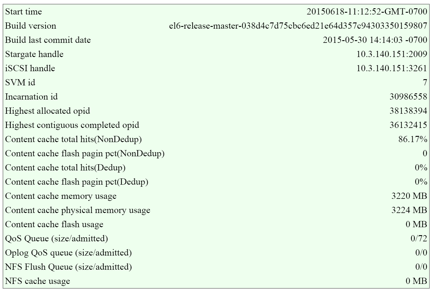
In this section there are two key areas I look out for, the first being the I/O queues that shows the number of admitted / outstanding operations.
The figure shows the queues portion of the overview section:

The second portion is the unified cache details that shows information on cache sizes and hit rates.
The figure shows the unified cache portion of the overview section:
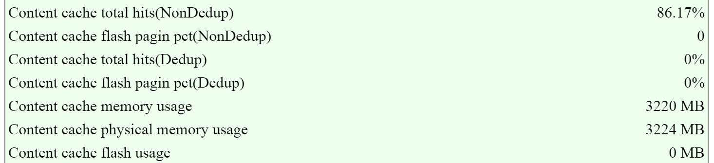
Note
Pro tip
In ideal cases the hit rates should be above 80-90%+ if the workload is read heavy for the best possible read performance.
NOTE: these values are per Stargate / CVM
The next section is the 'Cluster State' that shows details on the various Stargates in the cluster and their disk usages.
The figure shows the Stargates and disk utilization (available/total):
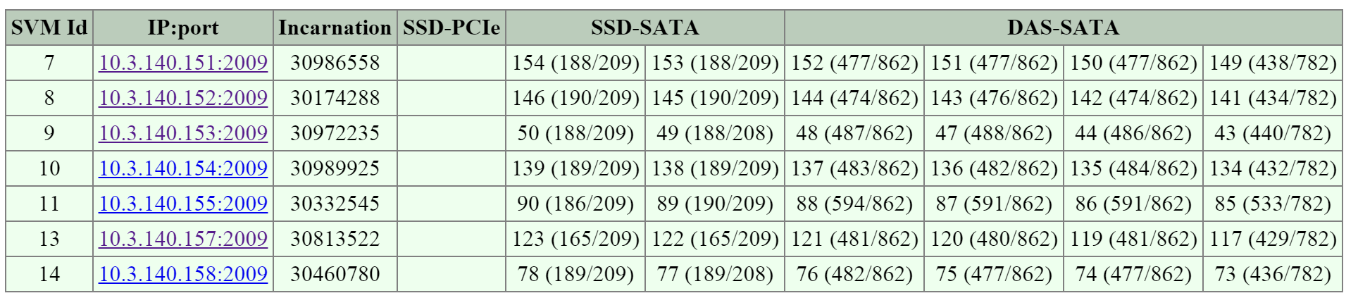
The next section is the 'NFS Slave' section which will show various details and stats per vDisk.
The figure shows the vDisks and various I/O details:
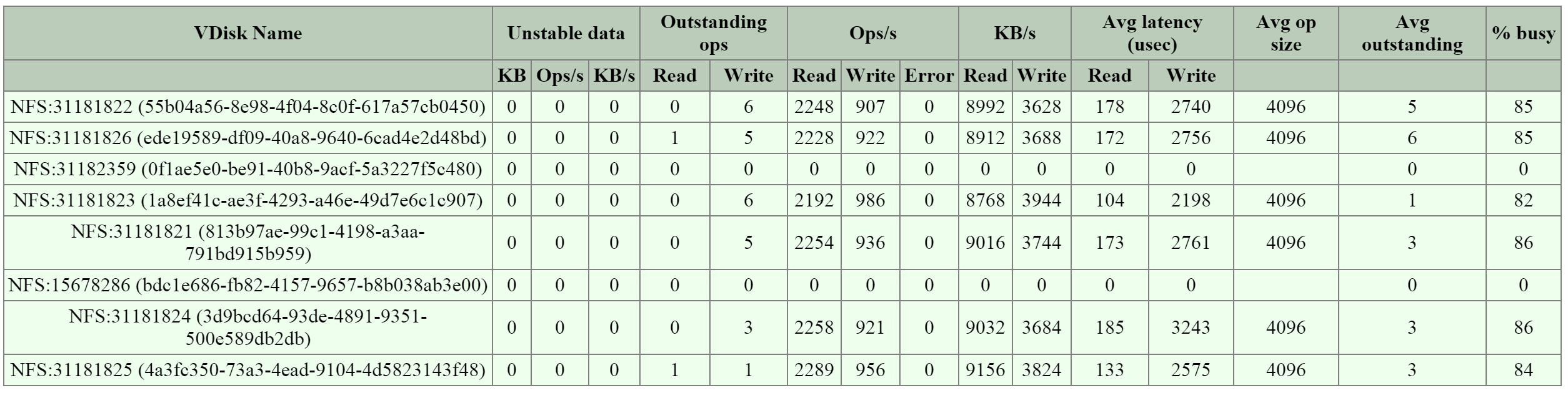
Note
Pro tip
When looking at any potential performance issues I always look at the following:
- Avg. latency
- Avg. op size
- Avg. outstanding
For more specific details the vdisk_stats page holds a plethora of information.
Using the 2009/vdisk_stats Page
The 2009 vdisk_stats page is a detailed page which provides even further data points per vDisk. This page includes details and a histogram of items like randomness, latency histograms, I/O sizes and working set details.
You can navigate to the vdisk_stats page by clicking on the 'vDisk Id' in the left hand column.
The figure shows the section and hyperlinked vDisk Id:
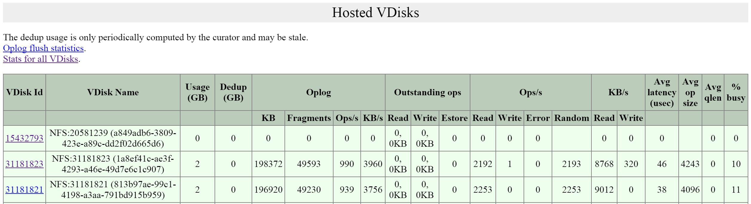
This will bring you to the vdisk_stats page which will give you the detailed vDisk stats. NOTE: These values are real-time and can be updated by refreshing the page.
The first key area is the 'Ops and Randomness' section which will show a breakdown of whether the I/O patterns are random or sequential in nature.
The figure shows the 'Ops and Randomness' section:
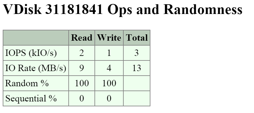
The next area shows a histogram of the frontend read and write I/O latency (aka the latency the VM / OS sees).
The figure shows the 'Frontend Read Latency' histogram:
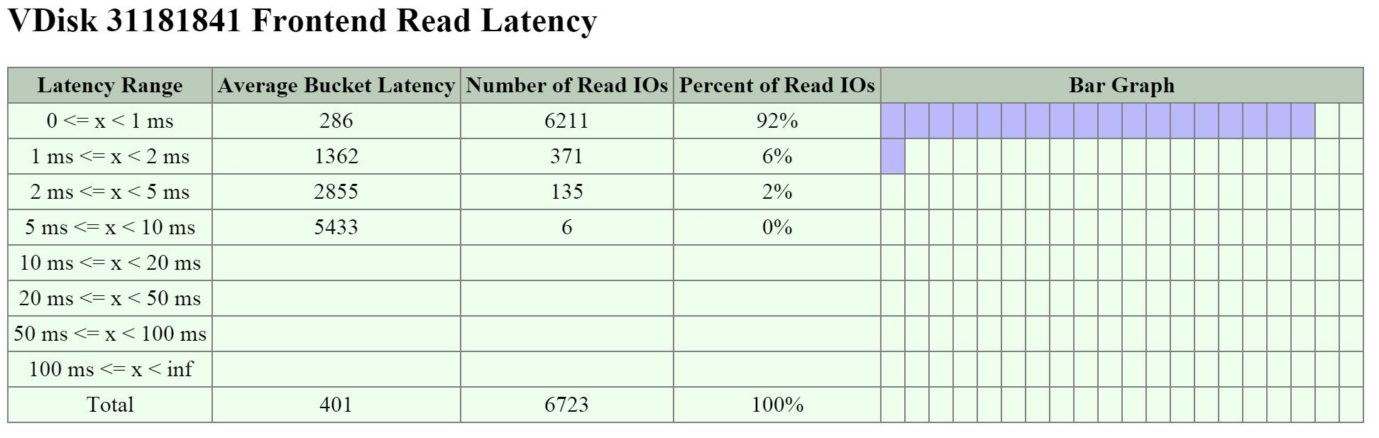
The figure shows the 'Frontend Write Latency' histogram:
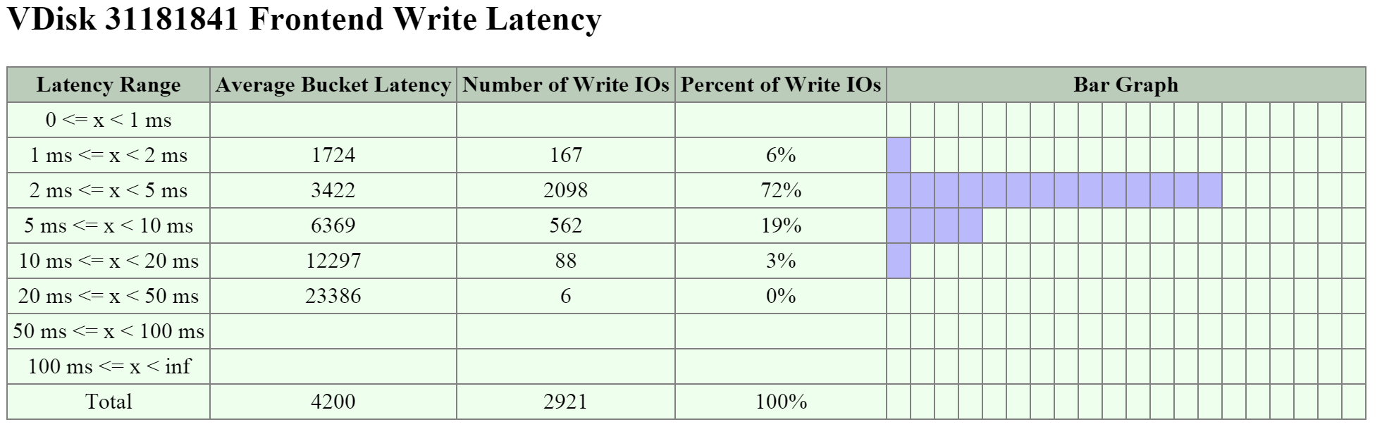
The next key area is the I/O size distribution that shows a histogram of the read and write I/O sizes.
The figure shows the 'Read Size Distribution' histogram:
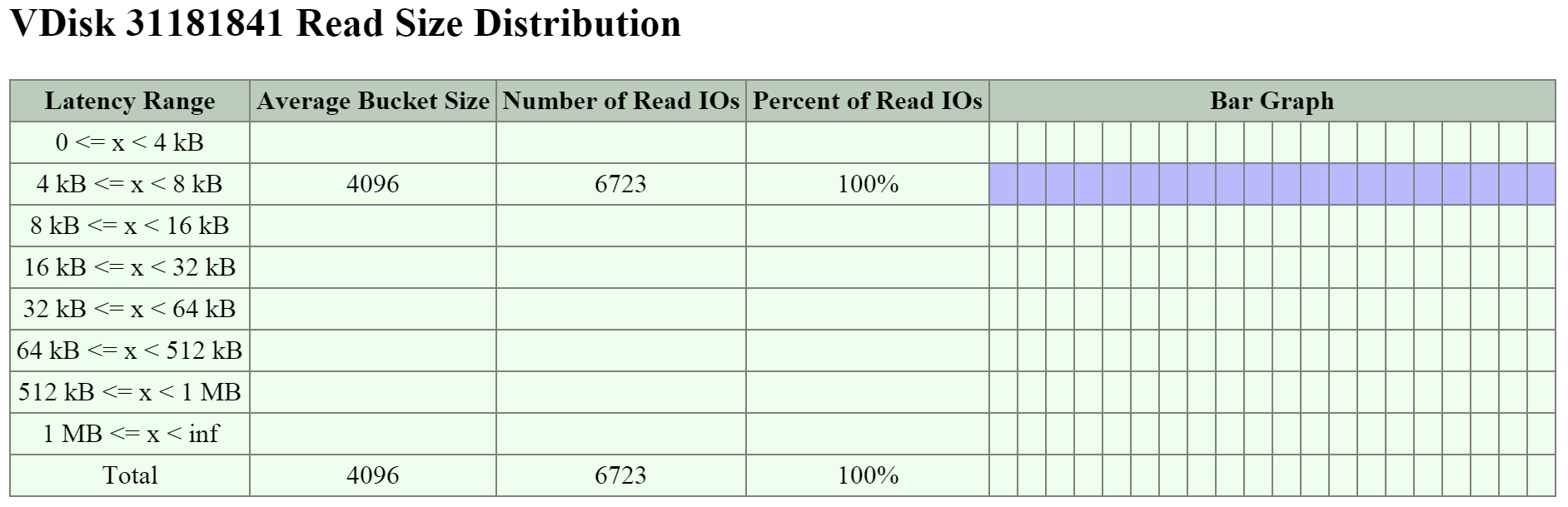
The figure shows the 'Write Size Distribution' histogram:
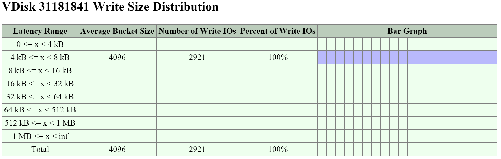
The next key area is the 'Working Set Size' section which provides insight on working set sizes for the last 2 minutes and 1 hour. This is broken down for both read and write I/O.
The figure shows the 'Working Set Sizes' table:
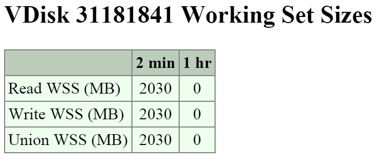
The 'Read Source' provides details on which tier or location the read I/Os are being served from.
The figure shows the 'Read Source' details:
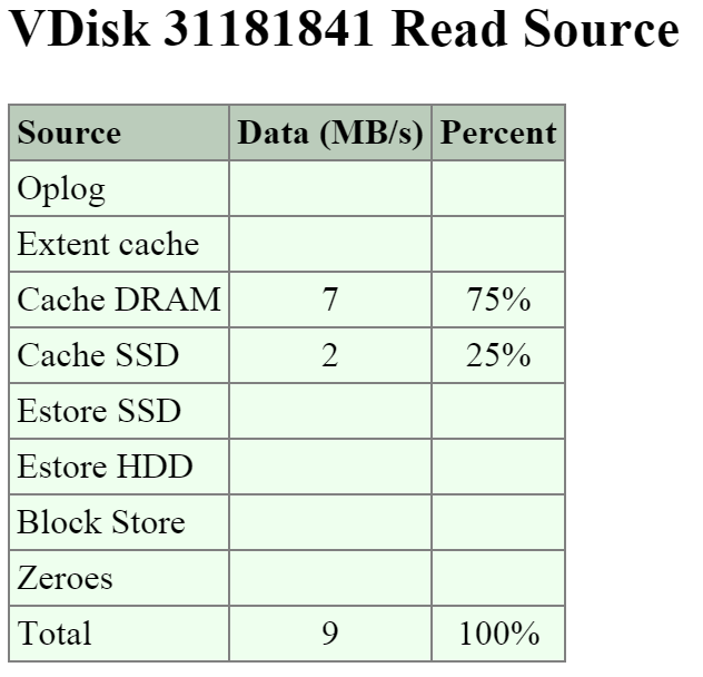
Note
Pro tip
If you're seeing high read latency take a look at the read source for the vDisk and take a look where the I/Os are being served from. In most cases high latency could be caused by reads coming from HDD (Estore HDD).
The 'Write Destination' section will show where the new write I/O are coming in to.
The figure shows the 'Write Destination' table:
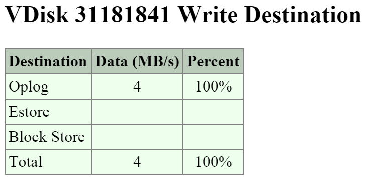
Note
Pro tip
Random I/Os will be written to the Oplog, sequential I/Os will bypass the Oplog and be directly written to the Extent Store (Estore).
Another interesting data point is what data is being up-migrated from HDD to SSD via ILM. The 'Extent Group Up-Migration' table shows data that has been up-migrated in the last 300, 3,600 and 86,400 seconds.
The figure shows the 'Extent Group Up-Migration' table:
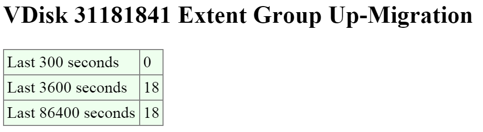
Using the 2010 Page (Curator)
The 2010 page is a detailed page for monitoring the Curator MapReduce framework. This page provides details on jobs, scans, and associated tasks.
You can navigate to the Curator page by navigating to http://<CVM IP>:2010. NOTE: if you're not on the Curator Master click on the IP hyperlink after 'Curator Master: '.
The top of the page will show various details about the Curator Master including uptime, build version, etc.
The next section is the 'Curator Nodes' table that shows various details about the nodes in the cluster, the roles, and health status. These will be the nodes Curator leverages for the distributed processing and delegation of tasks.
The figure shows the 'Curator Nodes' table:
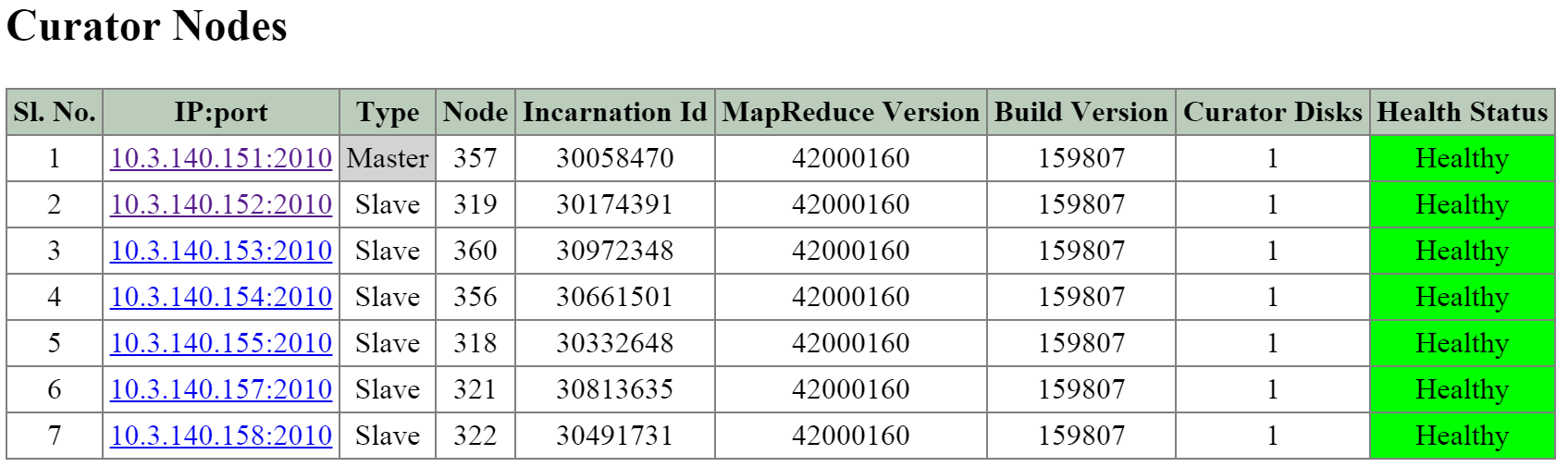
The next section is the 'Curator Jobs' table that shows the completed or currently running jobs.
There are two main types of jobs which include a partial scan which is eligible to run every 60 minutes and a full scan which is eligible to run every 6 hours. NOTE: the timing will be variable based upon utilization and other activities.
These scans will run on their periodic schedules however can also be triggered by certain cluster events.
Here are some of the reasons for a jobs execution:
- Periodic (normal state)
- Disk / Node / Block failure
- ILM Imbalance
- Disk / Tier Imbalance
The figure shows the 'Curator Jobs' table:
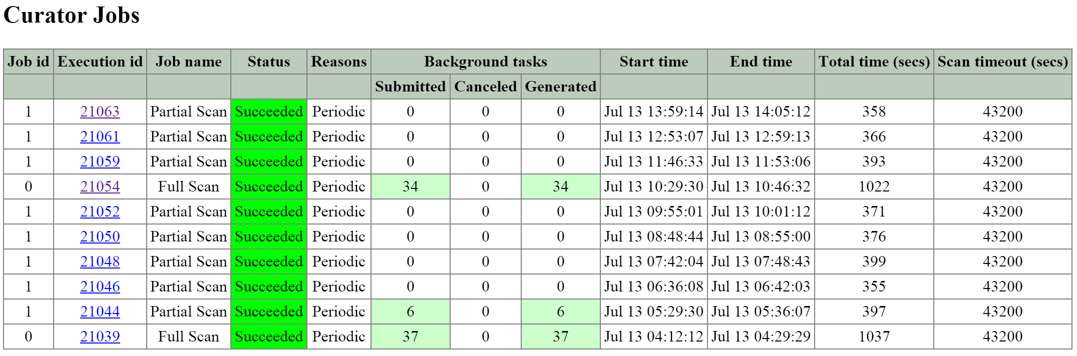
The table shows some of the high-level activities performed by each job:
| Activity | Full Scan | Partial Scan |
|---|---|---|
| ILM | X | X |
| Disk Balancing | X | X |
| Compression | X | X |
| Deduplication | X | |
| Erasure Coding | X | |
| Garbage Cleanup | X |
Clicking on the 'Execution id' will bring you to the job details page which displays various job stats as well as generated tasks.
The table at the top of the page will show various details on the job including the type, reason, tasks and duration.
The next section is the 'Background Task Stats' table which displays various details on the type of tasks, quantity generated and priority.
The figure shows the job details table:
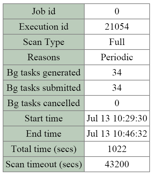
The figure shows the 'Background Task Stats' table:
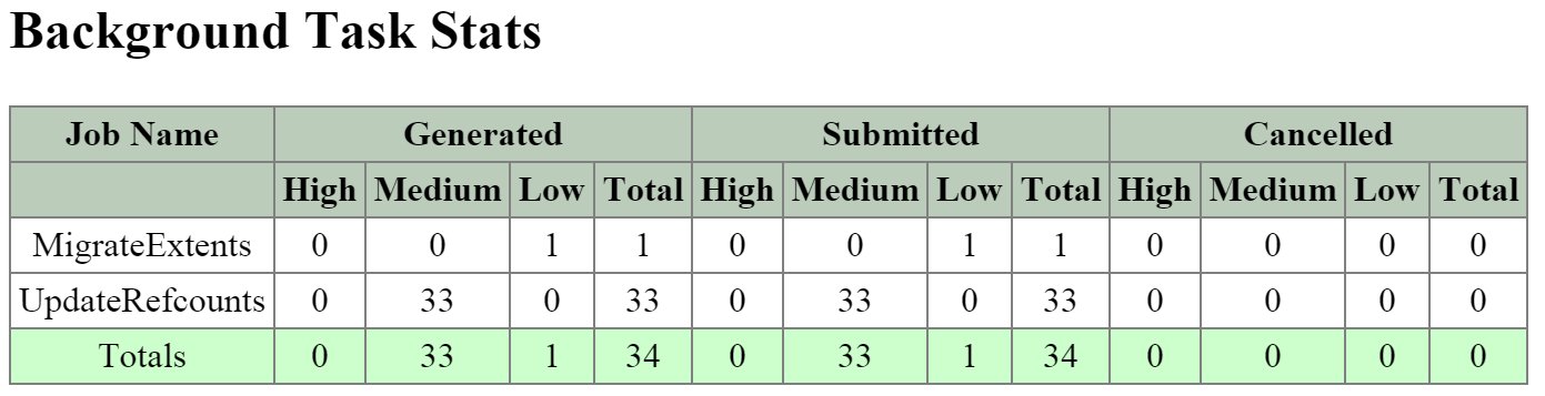
The next section is the 'MapReduce Jobs' table that shows the actual MapReduce jobs started by each Curator job. Partial scans will have a single MapReduce Job, full scans will have four MapReduce Jobs.
The figure shows the 'MapReduce Jobs' table:
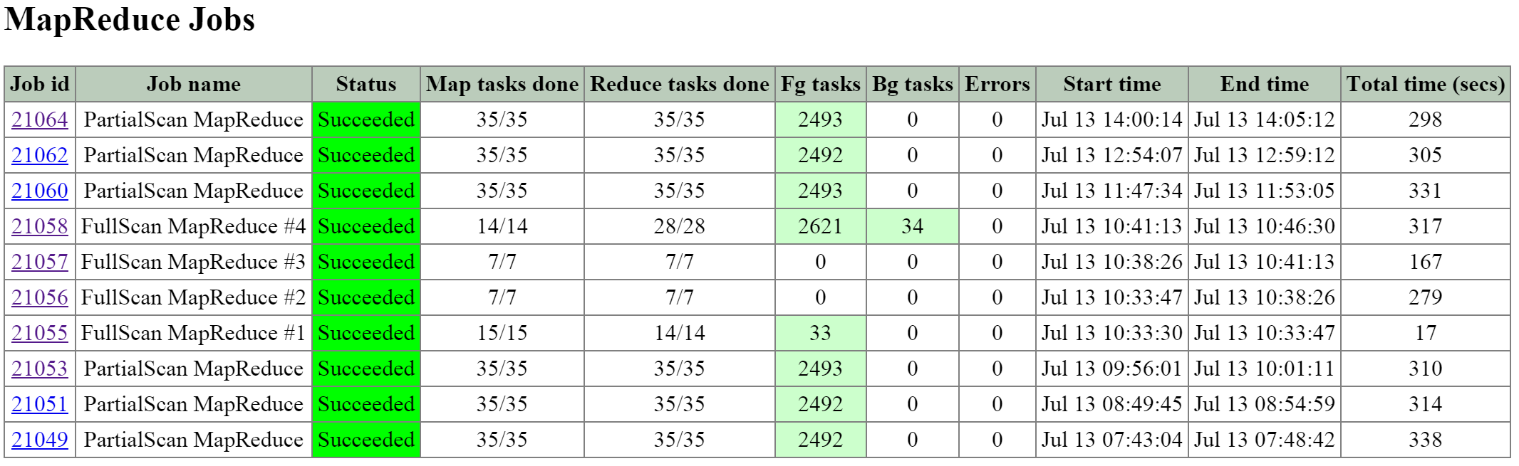
Clicking on the 'Job id' will bring you to the MapReduce job details page which displays the tasks status, various counters and details about the MapReduce job.
The figure shows a sample of some of the job counters:
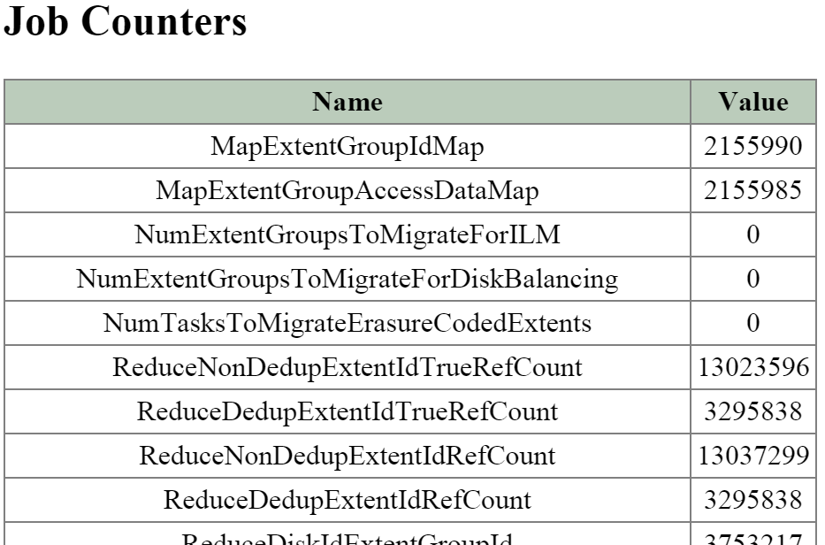
The next section on the main page is the 'Queued Curator Jobs' and 'Last Successful Curator Scans' section. These tables show when the periodic scans are eligible to run and the last successful scan's details.
The figure shows the 'Queued Curator Jobs' and 'Last Successful Curator Scans' section: